Fundamental of inequalities

Inequalities

Many mathematical descriptions of real situations are best expressed as inequalities rather than equations. For example, a firm might be able to use a machine no more than 12 hours a day, while production of at least 500 cases of a certain product might be required to meet a contract. The simplest way to see the solution of an inequality in two variables is to draw its graph.

  A line divides a plane into three sets of points: the points of the line itself and the points belonging to the two regions determined by the line. Each of these two regions is called a half-plane. In Figure 3.50 line r divides the plane into three different sets of points: line r, half-plane P, and half-plane Q. The points on r belong neither to P nor to Q. Line r is the boundary of each half-plane.

  A linear equality in two variables is an inequality of the form

  Ax+By<=C,

  Figure 3.50

  where A, B, and C are real numbers, with A and B not both equal to 0. (The symbol ≤ could be replaced with ≥ , <, or >.) The graph of a linear inequality is a half-plane, perhaps with its boundary. For example, to graph the linear inequality 3x -2y <= 6, first graph the boundary. 3x - 2y = 6, as shown in Figure 3.51.

  Since the points of the line 3x - 2y = 6 satisfy 3x -2y <= 6, this line is part of the solution. To decide which half-plane (the one above the line 3x - 2y = 6 or the one below the line) is part of the solution, solve the original inequality for y.

  3x-2y<=6

  -2y<=-3x+6

  y>=3/2x-3  Multiply by -1/2; change ≤ to ≥

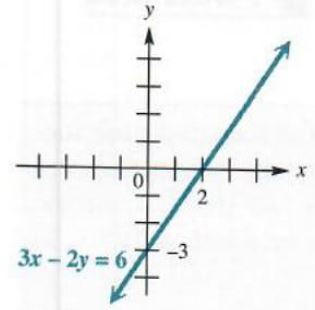
  Figure 3.51

  For a particular value of x, the inequality will be satisfied by all values of y that are greater than or equal to (3/2)x-3. This means that the solution includes the half-plane above the line, as well as the line itself. The domain and range are both (-∞,∞). See Figure 3.52.

  There is an alternative method for deciding which side of the boundary line to shade. Choose as a test point any point not on the graph of the equation. The origin, (0,0), is often a good test point (as long as it does not lie on the boundary line). Substituting 0 for x and 0 for y in the inequality 3x-2y<=6 gives

  3(0)-2(0)<=6

  0<=6

  a true statement. Since (0,0) leads to a true result, it is part of the solution of the inequality. Shade the side of the graph containing (0,0), as shown in Figure 3.52.

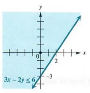
  Figure 3.52

Example 1

GRAPHING A LINEAR INEQUALITY

  Graph x+4y>4

  The boundary here is the straight line x + 4y = 4. Since the points on this line do not satisfy x + 4y > 4, it is customary to graph the boundary as a dashed line, as in Figure 3.53. To decide which half-plane satisfies the inequality, use a test point. Choosing (0,0) as a test point gives 0 + 4*0 > 4, or 0 > 4, a false statement. Since (0,0) leads to a false statement, shade the side of the graph not containing (0,0), as in Figure 3.53. 

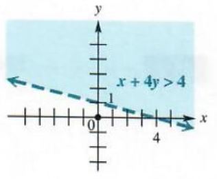
  Figure 3.53

Let’s see how our math solver generates graph for this and similar problems. Click on "Solve Similar" button to see more examples.

Example 2

GRAPHING A SECOND-DEGREE INEQUALITY

  Graph y=2x^2-3.

  First graph the boundary, the parabola y = 2x^2 - 3, as shown in Figure 3.54. Then select any test point not on the parabola, such as (0,0). Since (0,0) does not satisfy the original inequality, shade the portion of the graph that does not include (0,0), as shown in Figure 3.54. Because of the = portion of ≤ , the points on the parabola itself also belong to the graph. 

  Figure 3.54

NOTE

  Another method of determining the region to shade for a second-degree inequality that is solved for y is observing the inequality symbol. For instance, as in Example 2, since y is less than or equal lo 2x^2 - 3. we shade below the boundary. The graph of y>=2x^2-3 (y is greater than or equal to 2x^2 - 3 consists of the boundary and all points above it.

Let’s see how our math solver generates graph for this and similar problems. Click on "Solve Similar" button to see more examples.

Example 3

GRAPHING SECOND-DEGREE INEQUALITIES

  Graph each inequality

  (a) y^2<=1+4x^2

  Write the boundary y^2=1+4x^2 as y^2-4x^2=1, a hyperbola with y-intercepts 1 and -1. as shown in Figure 3.55(a). Select any point not on the hyperbola and test it in the original inequality. Since (0,0) satisfies this inequality, shade the area between the two branches of the hyperbola, as shown in Figure 3.55(a). The points on the hyperbola are part of the solution.

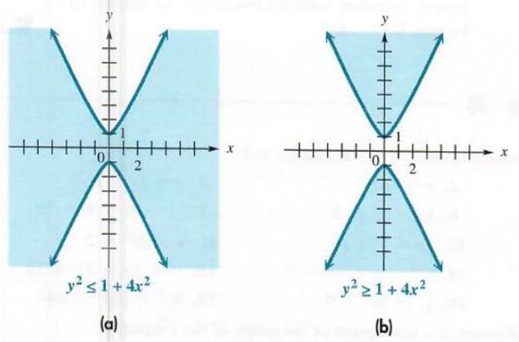
  Figure 3.55

Let’s see how our math solver generates graph for this and similar problems. Click on "Solve Similar" button to see more examples.

  (b) y^2>=1+4x^2

  The boundary is the same as in part (a). Since (0,0) makes this inequality false, the two regions above and below the branches of the hyperbola are shaded, as shown in Figure 3.55(b). Again, the points on the hyperbola itself are included in the solution. 

Example 4

GRAPHING A LINER INEQUALITY WITH A RESTRICTION

  Graph 2x-y<=4, where x<3.

  Figure 3.56 shows the graphs of both inequalities. The shaded area to the left of
the line x = 3 and above the line 2x - y = 4 represents the region that satisfies both inequalities. The point where the boundary lines intersect, (3, 2), belongs to the first inequality but not to the second. For this reason, (3, 2) is not part of the solution. This is shown with an open dot on the graph at (3, 2). 

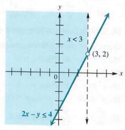
  Figure 3.56

Example 5

GRAPHING A SECOND-DEGREE INEQUALITY WITH A RESTRICTION

  Graph 16x^2+y^2<=16, where y>=0.

  The inequality 16x^2+y^2<=16 has as its boundary the ellipse 16x^2+y^2=16, partially graphed in Figure 3.57. Since the test point (0,0)satisfies the inequality, we shade inside the portion of the ellipse that is graphed. The inequality y>=0 includes all points on or above the x-axis. The final graph consists of the region inside the ellipse and above the x-axis, together with its boundary, as shown in Figure 3.57.

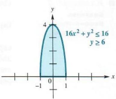
  Figure 3.57