Matrices

The matrices section of QuickMath allows you to perform arithmetic operations on matrices. Currently you can add or subtract matrices, multiply two matrices, multiply a matrix by a scalar and raise a matrix to any power.

What is a matrix?

A matrix is a rectangular array of elements (usually called scalars), which are set out in rows and columns. They have many uses in mathematics, including the transformation of coordinates and the solution of linear systems of equations.

Here is an example of a 2x3 matrix :

1   2   3

4   5   6

Arithmetic

The arithmetic suite of commands allows you to add or subtract matrices, carry out matrix multiplication and scalar multiplication and raise a matrix to any power.

Matrices are added to and subtracted from one another element by element. For instance, when adding two matrices A and B, the element at row i, column j of A is added to the element at row i, column j of B to give the element at row i, column j of the answer. Consequently, you can only add and subtract matrices which are the same size.

Matrix multiplication is a little more complicated. Suppose two matrices A and B are multiplied together to get a third matrix C. The element at row i, column j in C is found by taking row i from A and multiplying it by column j from B. Two matrices can only be multiplied together if the number of columns in the first equals the number of rows in the second.

Multiplying a matrix by a scalar simply involves multiplying each element by that scalar, whilst raising a matrix to a positive integer power can be achieved by a series of matrix multiplications.

There is currently no advanced arithmetic section, though this may be introduced in the future.

Go to the Arithmetic page

Inverse

The inverse command allows you to find the inverse of any non-singular, square matrix. The inverse of a square matrix A is another matrix B of the same size such that

A B = B A = I

where I is the identity matrix. The inverse of A is commonly written as A^-1.

Go to the Inverse page

Determinant

The determinant command allows you to find the determinant of any non-singular, square matrix.

For example, if A is a 3 x 3 matrix, then its determinant can be found as follows :

det(A) = a_1,1 A_1,1 - a_1,2 A_1,2 + a_1,3 A_1,3

where a_i,j is the element of A at row i, column j and A_i,j is the matrix constructed from A by removing row i and column j.

Go to the Determinant page

Introduction to Matrices and Systems of Equations

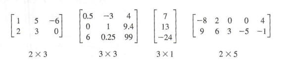
A matrix is a rectangular array of numbers arranged in rows and columns. We call each number in this array an element of the matrix. When we write a matrix, we typically enclose the array in brackets. Matrices (plural) come in many sizes, determined by the number of rows and the number of columns. If a matrix has n rows and m columns, then we say that the size of the matrix is m x n, read "m by n". The following are examples of matrices of various sizes.


When we enumerate rows and columns of a given matrix, we count rows from top to bottom and count columns from left to right.Since a matrix is an array of numbers, we often see matrices used to record information, especially if rows and columns of a matrix can be understood to represent categories. As such, we can certainly use matrices to record pertinent information about a system of linear equations - coefficients of the variables as well as constants on the right-hand side of equations in the system.

Consider the system

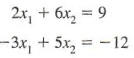
We adopt a convention here of using subscripted variables rather than individual letter variables to avoid possible difficulties in the number of available letters. We construct a 2 x 3 matrix, called the augmented matrix for the system, where each row represents information for a particular equation and each column represents either coefficients of a variable or the constants on the right-hand side of the equations.

We write this matrix as follows.



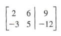
Notice the correspondence between the rows of this matrix and the equations in the system as well as the correspondence between the columns of the matrix and the coefficients and constant terms in the equations. The vertical line has no real purpose except to serve as a visual reminder of the location of the equal signs in the system and hence a separation between the coefficients of the variables and the constants on the right-hand side of the equations. Before delving into the use of these augmented matrices representing systems, we will pause to put forth some terminology and notation. Recall that in the method of elimination we had three operations that we could use to produce equivalent systems of linear equations. We have a similar collection of row operations that we perform on matrices. We say two matrices are row-equivalent if one is obtained from the other by some sequence of row operations. These operations are as follows:

Row Operations:

• Interchange any two rows.
• Multiply (all elements in) a row by any nonzero constant and replace that row with the result.
• Multiply (all elements in) a row by any constant and add (corresponding elements) to any other row, replacing the second row in this sum with the result.

Performing any sequence of these operations results in a row-equivalent matrix.

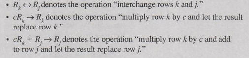
Notice the similarity between these operations and the operations employed in the method of elimination. We use a similar shorthand notation to indicate performing a particular row operation as well.

Notation for Row Operations

In the case where a matrix is the augmented matrix representing a system of linear equations, performing a row operation on the matrix is equivalent to performing the corresponding operation on a system of equations. So, row-equivalent matrices represent equivalent systems of linear equations. To demonstrate how to use augmented matrices to find solutions to systems of linear equations, we will show parallel operations in the method of elimination and the corresponding row operations.