FIRST-DEGREE EQUATIONS AND INEQUALITIES IN TWO VARIABLES
The language of mathematics is particularly effective in representing relationships between two or more variables. As an example, let us consider the distance traveled in a certain length of time by a car moving at a constant speed of 40 miles per hour. We can represent this relationship by
- 1. A word sentence:
The distance traveled in miles is equal to forty times the number of hours traveled. - 2. An equation:
d = 40r. - 3. A tabulation of values.
- 4. A graph showing the relationship between time and distance.
We have already used word sentences and equations to describe such relationships; in this chapter, we will deal with tabular and graphical representations.
7.1 SOLVING EQUATIONS IN TWO VARIABLES
ORDERED PAIRS
The equation d = 40f pairs a distance d for each time t. For example,
if t = 1, then d = 40
if t = 2, then d = 80
if t = 3, then d = 120
and so on.
The pair of numbers 1 and 40, considered together, is called a solution of the equation d = 40r because when we substitute 1 for t and 40 for d in the equation, we get a true statement. If we agree to refer to the paired numbers in a specified order in which the first number refers to time and the second number refers to distance, we can abbreviate the above solutions as (1, 40), (2, 80), (3, 120), and so on. We call such pairs of numbers ordered pairs, and we refer to the first and second numbers in the pairs as components. With this agreement, solutions of the equation d - 40t are ordered pairs (t, d) whose components satisfy the equation. Some ordered pairs for t equal to 0, 1, 2, 3, 4, and 5 are
(0,0), (1,40), (2,80), (3,120), (4,160), and (5,200)
Such pairings are sometimes shown in one of the following tabular forms.

In any particular equation involving two variables, when we assign a value to one of the variables, the value for the other variable is determined and therefore dependent on the first. It is convenient to speak of the variable associated with the first component of an ordered pair as the independent variable and the variable associated with the second component of an ordered pair as the dependent variable. If the variables x and y are used in an equation, it is understood that replace- ments for x are first components and hence x is the independent variable and replacements for y are second components and hence y is the dependent variable. For example, we can obtain pairings for equation

by substituting a particular value of one variable into Equation (1) and solving for the other variable.
Example 1
Find the missing component so that the ordered pair is a solution to
2x + y = 4
a. (0,?)
b. (1,?)
c. (2,?)
Solution
if x = 0, then 2(0) + y = 4
y = 4
if x = 1, then 2(1) + y = 4
y = 2
if x = 2, then 2(2) + y = 4
y = 0
The three pairings can now be displayed as the three ordered pairs
(0,4), (1,2), and (2,0)
or in the tabular forms

EXPRESSING A VARIABLE EXPLICITLY
We can add -2x to both members of 2x + y = 4 to get
-2x + 2x + y = -2x + 4
y = -2x + 4
In Equation (2), where y is by itself, we say that y is expressed explicitly in terms of x. It is often easier to obtain solutions if equations are first expressed in such form because the dependent variable is expressed explicitly in terms of the independent variable.
For example, in Equation (2) above,
if x = 0, then y = -2(0) + 4 = 4
if x = 1, then y = -2(1) + 4 = 2
if x = 2 then y = -2(2) + 4 = 0
We get the same pairings that we obtained using Equation (1)
(0,4), (1,2), and (2,0)
We obtained Equation (2) by adding the same quantity, -2x, to each member of Equation (1), in that way getting y by itself. In general, we can write equivalent equations in two variables by using the properties we introduced in Chapter 3, where we solved first-degree equations in one variable.
Equations are equivalent if:
- The same quantity is added to or subtracted from equal quantities.
- Equal quantities are multiplied or divided by the same nonzero quantity.
Example 2
Solve 2y - 3x = 4 explicitly for y in terms of x and obtain solutions for x = 0, x = 1, and x = 2.
Solution
First, adding 3x to each member we get
2y - 3x + 3x = 4 + 3x
2y = 4 + 3x (continued)
Now, dividing each member by 2, we obtain

In this form, we obtain values of y for given values of x as follows:

In this case, three solutions are (0, 2), (1, 7/2), and (2, 5).
FUNCTION NOTATION
Sometimes, we use a special notation to name the second component of an ordered pair that is paired with a specified first component. The symbol f(x), which is often used to name an algebraic expression in the variable x, can also be used to denote the value of the expression for specific values of x. For example, if
f(x) = -2x + 4
where f{x) is playing the same role as y in Equation (2) on page 285, then f(1) represents the value of the expression -2x + 4 when x is replaced by 1
f(l) = -2(1) + 4 = 2
Similarly,
f(0) = -2(0) + 4 = 4
and
f(2) = -2(2) + 4 = 0
The symbol f(x) is commonly referred to as function notation.
Example 3
If f(x) = -3x + 2, find f(-2) and f(2).
Solution
Replace x with -2 to obtain
f(-2) = -3(-2) + 2 = 8
Replace x with 2 to obtain
f(2) = -3(2) + 2 = -4
7.2 GRAPHS OF ORDERED PAIRS
In Section 1.1, we saw that every number corresponds to a point in a line. Simi- larly, every ordered pair of numbers (x, y) corresponds to a point in a plane. To graph an ordered pair of numbers, we begin by constructing a pair of perpendicular number lines, called axes. The horizontal axis is called the x-axis, the vertical axis is called the y-axis, and their point of intersection is called the origin. These axes divide the plane into four quadrants, as shown in Figure 7.1.

Now we can assign an ordered pair of numbers to a point in the plane by referring to the perpendicular distance of the point from each of the axes. If the first component is positive, the point lies to the right of the vertical axis; if negative, it lies to the left. If the second component is positive, the point lies above the horizontal axis; if negative, it lies below.
Example 1
Graph (3, 2), (-3, 2), (-3, -2), and (3, -2) on a rectangular coordinate system.
Solution
The graph of (3, 2) lies 3 units to the right of
the y-axis and 2 units above the x-axis;
the graph of (-3,2) lies 3 units to the left of the
y-axis and 2 units above the x-axis;
the graph of (-3, -2) lies 3 units to the left of
the y-axis and 2 units below the x-axis;
the graph of (3, -2) lies 3 units to the right of
the y-axis and 2 units below the x-axis.

The distance y that the point is located from the x-axis is called the ordinate of the point, and the distance x that the point is located from the y-axis is called the abscissa of the point. The abscissa and ordinate together are called the rectan- gular or Cartesian coordinates of the point (see Figure 7.2).

7.3 GRAPHING FIRST-DEGREE EQUATIONS
In Section 7.1, we saw that a solution of an equation in two variables is an ordered pair. In Section 7.2, we saw that the components of an ordered pair are the coordinates of a point in a plane. Thus, to graph an equation in two variables, we graph the set of ordered pairs that are solutions to the equation. For example, we can find some solutions to the first-degree equation
y = x + 2
by letting x equal 0, -3, -2, and 3. Then,
for x = 0, y=0+2=2
for x = 0, y = -3 + 2 = -1
for x = -2, y = -2 + 2 - 0
for x = 3, y = 3 + 2 = 5
and we obtain the solutions
(0,2), (-3,-1), (-2,0), and (3,5)
which can be displayed in a tabular form as shown below.

If we graph the points determined by these ordered pairs and pass a straight line through them, we obtain the graph of all solutions of y = x + 2, as shown in Figure 7.3. That is, every solution of y = x + 2 lies on the line, and every point on the line is a solution of y = x + 2.

The graphs of first-degree equations in two variables are always straight lines; therefore, such equations are also referred to as linear equations.
In the above example, the values we used for x were chosen at random; we could have used any values of x to find solutions to the equation. The graphs of any other ordered pairs that are solutions of the equation would also be on the line shown in Figure 7.3. In fact, each linear equation in two variables has an infinite number of solutions whose graph lies on a line. However, we only need to find two solutions because only two points are necessary to determine a straight line. A third point can be obtained as a check.
To graph a first-degree equation:
- Construct a set of rectangular axes showing the scale and the variable repre- sented by each axis.
- Find two ordered pairs that are solutions of the equation to be graphed by assigning any convenient value to one variable and determining the corre- sponding value of the other variable.
- Graph these ordered pairs.
- Draw a straight line through the points.
- Check by graphing a third ordered pair that is a solution of the equation and verify that it lies on the line.
Example 1
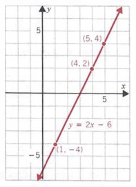
Graph the equation y = 2x - 6.
Solution
We first select any two values of x to find the associated values of y.
We will use 1 and 4 for x.
If x = 1, y = 2(1) - 6 = -4
if x = 4, y = 2(4) - 6 = 2
Thus, two solutions of the equation are
(1, -4) and (4, 2).
Next, we graph these ordered pairs and draw a straight line through the points as shown
in the figure. We use arrowheads to show that
the line extends infinitely far in both directions.
Any third ordered pair that satisfies the
equation can be used as a check:
if x = 5, y = 2(5) -6 = 4
We then note that the graph of (5, 4) also lies on the line
To find solutions to an equation, as we have noted it is often easiest to first solve
explicitly for y in terms of x.
Example 2
Graph x + 2y = 4.
Solution
We first solve for y in terms of x to get

We now select any two values of x to find the associated values of y. We will use 2 and 0 for x.

Thus, two solutions of the equation are (2, 1) and (0, 2).
Next, we graph these ordered pairs and pass a straight line through the points, as shown in the figure.
Any third ordered pair that satisfies the equation can be used as a check:


We then note that the graph of (-2, 3) also lies on the line.
SPECIAL CASES OF LINEAR EQUATIONS
The equation y = 2 can be written as
0x + y = 2
and can be considered a linear equation in two variables where the coefficient of x is 0. Some solutions of 0x + y = 2 are
(1,2), (-1,2), and (4,2)
In fact, any ordered pair of the form (x, 2) is a solution of (1). Graphing the solutions yields a horizontal line as shown in Figure 7.4.

Similarly, an equation such as x = -3 can be written as
x + 0y = -3
and can be considered a linear equation in two variables where the coefficient of y is 0.
Some solutions of x + 0y = -3 are (-3, 5), (-3, 1), and (-3, -2). In fact, any ordered pair of the form (-3, y) is a solution of (2). Graphing the solutions yields a vertical line as shown in Figure 7.5.

Example 3
Graph
a. y = 3
b. x=2
Solution
a. We may write y = 3 as Ox + y =3.
Some solutions are (1, 3), (2,3), and (5, 3).

b. We may write x = 2 as x + Oy = 2.
Some solutions are (2, 4), (2, 1), and (2, -2).

7.4 INTERCEPT METHOD OF GRAPHING
In Section 7.3, we assigned values to x in equations in two variables to find the corresponding values of y. The solutions of an equation in two variables that are generally easiest to find are those in which either the first or second component is 0. For example, if we substitute 0 for x in the equation
3x + 4y = 12
we have
3(0) + 4y = 12
y = 3
Thus, a solution of Equation (1) is (0, 3). We can also find ordered pairs that are solutions of equations in two variables by assigning values to y and determining the corresponding values of x. In particular, if we substitute 0 for y in Equation (1), we get
3x + 4(0) = 12
x = 4
and a second solution of the equation is (4, 0). We can now use the ordered pairs (0, 3) and (4, 0) to graph Equation (1). The graph is shown in Figure 7.6. Notice that the line crosses the x-axis at 4 and the y-axis at 3. For this reason, the number 4 is called the x-intercept of the graph, and the number 3 is called the y-intercept.

This method of drawing the graph of a linear equation is called the intercept method of graphing. Note that when we use this method of graphing a linear equation, there is no advantage in first expressing y explicitly in terms of x.
Example 1
Graph 2x - y = 6 by the intercept method.
Solution
We find the x-intercept by substituting 0 for y in the equation to obtain
2x - (0) = 6
2x = 6
x = 3
Now, we find the y-intercept by substituting for x in the equation to get
2(0) - y = 6
-y = 6
y = -6
The ordered pairs (3, 0) and (0, -6) are solutions of 2x - y = 6. Graphing these points and connecting them with a straight line give us the graph of 2x - y = 6. If the graph intersects the axes at or near the origin, the intercept method is not satisfactory. We must then graph an ordered pair that is a solution of the equation and whose graph is not the origin or is not too close to the origin.

Example 2
Graph y = 3x.
Solution
We can substitute 0 for x and find
y = 3(0) = 0
Similarly, substituting 0 for y, we get
0 = 3.x, x = 0
Thus, 0 is both the x-intercept and the y-intercept.
Since one point is not sufficient to graphy = 3x, we resort to the methods outlined in Section 7.3. Choosing any other value for x,say 2, we get
y = 3(2) = 6
Thus, (0, 0) and (2, 6) are solutions to the equation. The graph of y = 3x is shown at the right.

7.5 SLOPE OF A LINE
SLOPE FORMULA
In this section, we will study an important property of a line. We will assign a number to a line, which we call slope, that will give us a measure of the "steepness" or "direction" of the line.
It is often convenient to use a special notation to distinguish between the rectan- gular coordinates of two different points. We can designate one pair of coordinates by (x1, y1 (read "x sub one, y sub one"), associated with a point P1, and a second pair of coordinates by (x2, y2), associated with a second point P2, as shown in Figure 7.7. Note in Figure 7.7 that when going from P1 to P2, the vertical change (or vertical distance) between the two points is y2 - y1 and the horizontal change (or horizontal distance) is x2 - x1.

The ratio of the vertical change to the horizontal change is called the slope of the line containing the points P1 and P2. This ratio is usually designated by m. Thus,

Example 1
Find the slope of the line containing the two points with coordinates (-4, 2) and (3, 5) as shown in the figure at the right.
Solution
We designate (3, 5) as (x2, y2) and (-4, 2)
as (x1, y1). Substituting into Equation (1)
yields

Note that we get the same result if we subsitute -4 and 2 for x2 and y2 and 3 and 5 for x1 and y1

Lines with various slopes are shown in Figure 7.8 below. Slopes of the lines that go up to the right are positive (Figure 7.8a) and the slopes of lines that go down to the right are negative (Figure 7.8b). And note (Figure 7.8c) that because all points on a horizontal line have the same y value, y2 - y1 equals zero for any two points and the slope of the line is simply

Also note (Figure 7.8c) that since all points on a vertical have the same x value, x2 - x1 equals zero for any two points. However,

is undefined, so that a vertical line does not have a slope.

PARALLEL AND PERPENDICULAR LINES
Consider the lines shown in Figure 7.9. Line l1 has slope m1 = 3, and line l2 has slope m2 = 3. In this case,

These lines will never intersect and are called parallel lines. Now consider the lines shown in Figure 7.10. Line l1, has slope m1 = 1/2 and line l2 has slope m2 = -2. In this case,

These lines meet to form a right angle and are called perpendicular lines.

In general, if two lines have slopes and m2:
-
a. The lines are parallel if they have the same slope, that is,
if m1 = m2.
b. The lines are perpendicular If the product of their slopes is -1, that is, if m1 * m2 = -1.
7.6 EQUATIONS OF STRAIGHT LINES
POINT-SLOPE FORM
In Section 7.5, we found the slope of a straight line by using the formula

Let us say we know that a line goes through the point (2, 3) and has a slope of 2. If we denote any other point on the line as P(x, y) (See Figure 7.1 la), by the slope formula

Thus, Equation (1) is the equation of the line that goes through the point (2, 3) and has a slope of 2.

In general let us say we know a line passes through a point P1(x1, y1 and has slope m. If we denote any other point on the line as P(x, y) (see Figure 7.11 b), by the slope formula

Equation (2) is called the point-slope form for a linear equation. In Equation (2), m, x1 and y1 are known and x and y are variables that represent the coordinates of any point on the line. Thus, whenever we know the slope of a line and a point on the line, we can find the equation of the line by using Equation (2).
Example 1
A line has slope -2 and passes through point (2, 4). Find the equation of the line.
Solution
Substitute -2 for m and (2, 4) for (x1, y1) in Equation (2)

Thus, a line with slope -2 that passes through the point (2, 4) has the equation y = -2x + 8. We could also write the equation in equivalent forms y + 2x = 8, 2x + y = 8, or 2x + y - 8 = 0.
SLOPE-INTERCEPT FORM
Now consider the equation of a line with slope m and y-intercept b as shown in Figure 7.12. Substituting 0 for x1 and b for y1 in the point-slope form of a linear equation, we have
y - b = m(x - 0)
y - b = mx
or
y = mx + b
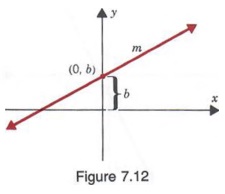
Equation (3) is called the slope-intercept form for a linear equation. The slope and y-intercept can be obtained directly from an equation in this form.
Example 2 If a line has the equation

then the slope of the line must be -2 and the y-intercept must be 8. Similarly, the graph of
y = -3x + 4
has a slope -3 and a y-intercept 4; and the graph of

has a slope 1/4 and a y-intercept -2.
If an equation is not written in x = mx + b form and we want to know the slope and/or the y-intercept, we rewrite the equation by solving for y in terms of x.
Example 3
Find the slope and y-intercept of 2x - 3y = 6.
Solution
We first solve for y in terms of x by adding -2x to each member.
2x - 3y - 2x = 6 - 2x
- 3y = 6 - 2x
Now dividing each member by -3, we have

Comparing this equation with the form y = mx + b, we note that the slope m (the coefficient of x) equals 2/3, and the y-intercept equals -2.
7.7 DIRECT VARIATION
A special case of a first-degree equation in two variables is given by
y = kx (k is a constant)
Such a relationship is called a direct variation. We say that the variable y varies directly as x.
Example 1
We know that the pressure P in a liquid varies directly as the depth d below the surface of the liquid. We can state this relationship in symbols as
P = kd
In a direct variation, if we know a set of conditions on the two variables, and if we further know another value for one of the variables, we can find the value of the second variable for this new set of conditions.
In the above example, we can solve for the constant k to obtain

Since the ratio P/d is constant for each set of conditions, we can use a proportion to solve problems involving direct variation.
Example 2
If pressure P varies directly as depth d, and P = 40 when d = 10, find P when d = 15.
Solution
Since the ratio P/d is constant, we can substitute values for P and d and obtain the
proportion

Thus, P = 60 when d = 15.
7.8 INEQUALITIES IN TWO VARIABLES
In Sections 7.3 and 7.4, we graphed equations in two variables. In this section we will graph inequalities in two variables. For example, consider the inequality
y ≤ -x + 6
The solutions are ordered pairs of numbers that "satisfy" the inequality. That is, (a, b) is a solution of the inequality if the inequality is a true statement after we substitute a for x and b for y.
Example 1
Determine if the given ordered pair is a solution of y = -x + 6.
a. (1, 1)
b. (2, 5)
Solution
The ordered pair (1, 1) is a solution because, when 1 is substituted for x and 1 is
substituted for y, we get
(1) = -(1) + 6, or 1 = 5
which is a true statement. On the other hand, (2, 5) is not a solution because when 2 is substituted for x and 5 is substituted for y, we obtain
(5) = -(2) + 6, or 5 = 4
which is a false statement.
To graph the inequality y = -x + 6, we first graph the equation y = -x + 6 shown in Figure 7.13. Notice that (3, 3), (3, 2), (3, 1), (3, 0), and so on, associated with the points that are on or below the line, are all solutions of the inequality y = -x + 6, whereas (3,4), (3, 5), and (3,6), associated with points above the line are not solutions of the inequality. In fact, all ordered pairs associated with points on or below the line are solutions of y = - x + 6. Thus, every point on or below the line is in the graph. We represent this by shading the region below the line (see Figure 7.14).

In general, to graph a first-degree inequality in two variables of the form Ax + By = C or Ax + By = C, we first graph the equation Ax + By = C and then determine which half-plane (a region above or below the line) contains the solutions. We then shade this half-plane. We can always determine which half- plane to shade by selecting a point (not on the line of the equation Ax + By = C) and testing to see if the ordered pair associated with the point is a solution of the given inequality. If so, we shade the half-plane containing the test point; otherwise, we shade the other half-plane. Often, (0, 0) is a convenient test point.
Example 2
Graph 2x+3y = 6
Solution
We first graph the line 2x + 3y = 6 (see graph a). Using the origin as a test point,
we determine whether (0, 0) is a solution of 2x + 3y ≥ 6. Since the statement
2(0) + 3(0) = 6
is false, (0, 0) is not a solution and we shade the half-plane that does not contain the origin (see graph b).

When the line Ax + By = C passes through the origin, (0, 0) is not a valid test point since it is on the line.
Example 3
Graph y = 2x.
Solution
We begin by graphing the line y = 2x (see graph a). Since the line passes through
the origin, we must choose another point not on the line as our test point. We will
use (0, 1). Since the statement
(1) = 2(0)
is true, (0, 1) is a solution and we shade the half-plane that contains (0, 1) (see graph b).

If the inequality symbol is '< or > , the points on the graph of Ax + By = C are not solutions of the inequality. We then use a dashed line for the graph of Ax + By = C.
CHAPTER SUMMARY
A solution of an equation in two variables is an ordered pair of numbers. In the ordered pair (x, y), x is called the first component and y is called the second component. For an equation in two variables, the variable associated with the first component of a solution is called the independent variable and the variable associated with the second component is called the dependent variable. Function notation f(x) is used to name an algebraic expression in x. When x in the symbol f(x) is replaced by a particular value, the symbol represents the value of the expression for that value of x.
The intersection of the two perpendicular axes in a coordinate systemis called the origin of the system, and each of the four regions into which the plane is divided is called a quadrant. The components of an ordered pair (x, y) associated with a point in the plane are called the coordinates of the point; x is called the abscissa of the point and y is called the ordinate of the point.
The graph of a first-degree equation in two variables is a straight line. That is, every ordered pair that is a solution of the equation has a graph that lies in a line, and every point in the line is associated with an ordered pair that is a solution of the equation.
The graphs of any two solutions of an equation in two variables can be used to obtain the graph of the equation. However, the two solutions of an equation in two variables that are generally easiest to find are those in which either the first or second component is 0. The x-coordinate of the point where a line crosses the x-axis is called the x-intercept of the line, and the y-coordinate of the point where a line crosses the y-axis is called they-intercept of the line. Using the intercepts to graph an equation is called the intercept method of graphing.
The slope of a line containing the points P1(x1, y1) and P2(x2, y2) is given by
![]()
Two lines are parallel if they have the same slope (m1 = m2).
Two lines are perpendicular if the product of their slopes is - l(m1 * m2 = -1).
The point-slope form of a line with slope m and passing through the point (x1, y1) is
y - y1 - m(x - x1)
The slope-intercept form of a line with slope m and y-intercept b is
y = mx + b
A relationship determined by an equation of the form
y = kx (k a constant)
is called a direct variation.
A solution of an inequality in two variables is an ordered pair of numbers that, when substituted into the inequality, makes the inequality a true statement. The graph of a linear inequality in two variables is a half-plane. The symbols introduced in this chapter appear on the inside front covers.
