Exponentials and Logarithms
Exponential Functions and Logarithms
10.1 Real Exponents
Recall from Chapter 5 that if a is a positive real number, then a^x is defined for each positive integer x. Later in the chapter, the set of exponents was extended to include, first, all integers and, next, all rational numbers. In this section we will consider the extension of the set of exponents to all real numbers. Although a careful definition of expressions such as 3^(root(2)) is beyond the scope of this book, we can develop an intuitive understanding of real exponents by considering the graphs of some specific examples.
Example 1. Graph y=2^x
We tabulate points only for rational values of x, since at this stage 2^x is known only for such x.
| x | 2x |
| -3 |
2^-3=1/8 |
| -2 | 2^-2=1/4 |
| -3/2 | 2^(-3/2)=1/(2root(2))=(root(2))/(4)≈0.4 |
| -1 | 2^-1=1/2 |
| -1/2 | 2^(-1/2)=1/(root(2))≈0.7 |
| 0 | 2^0=1 |
| 1/2 | 2^(1/2)=root(2)≈1.4 |
| 1 | 2^1=2 |
| 3/2 | 2^(3/2)=2root(2)≈2.8 |
| 2 | 2^2=4 |
| 3 | 2^3=8 |
Note that table A is used to obtain 2^(1/2)=root(2)≈1.4. The points in the table are plotted on a coordinate plane and connected with a smooth curve. (See Figure 1.)
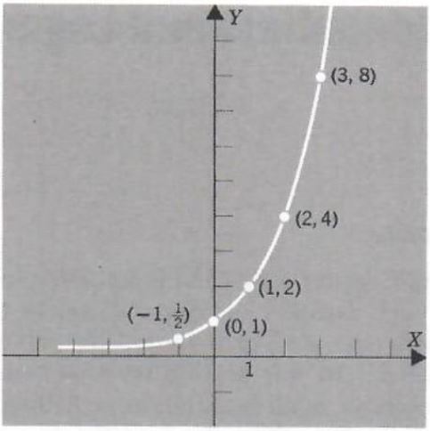
Figure 1.
From Figure 1 it appears reasonable that each horizontal line through a point on the positive Y axis intersects the curve in exactly one point. This gives us the property that for each positive real number Y there is exactly one real number xsuch that 2^x=y. Another way of stating this property is that if 2^a=2^b, then a=b.
As in Chapter 7, the graph may be used to estimate the value of 2^x for any real number x. Furthermore, for a given positive number b the graph may be used to estimate the real number x such that 2^x=b. The property above guarantees that there is exactly one such x.
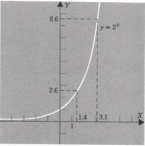
Figure 2.
Example 2. Estimate 2^(root(2) and 2^PI
We first draw the graph ofy=2^x (see Figure 2).
Since root(2) ≈ 1.4 and PI ≈ 3.1, from the graph ofy=2^x we have
2^(root(2))≈2^(1.4)
≈2.6
2^PI≈2^(3.1)
≈8.6
Example 3. Solve each of the following equations: (a) 2^x=8 (b) 2^x=1/16 (c) 2^x=7
(a) 2^x=8
Since 8=2^3, we have
2^x=2^3
x=3
(b) 2^x=1/16
Since 1/16=1/(2^4)=2^(-4), we have
2^x=2^(-4)
x=-4
(c) 2^x=7
Since 7 cannot be written as 2to a rational exponent, we use the graph in Figure 3 to approximate the solution.
Thus,
x≈ 2.8

Figure 3.
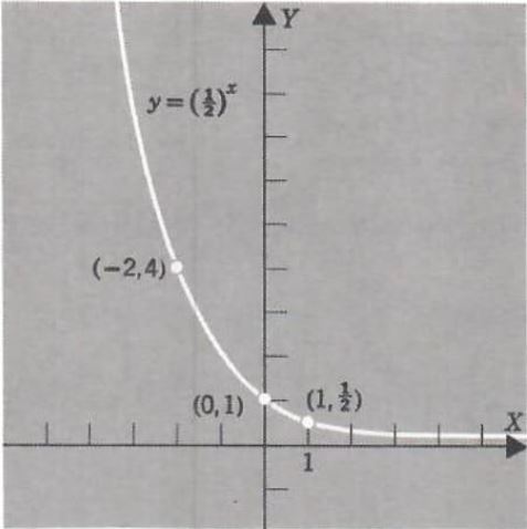
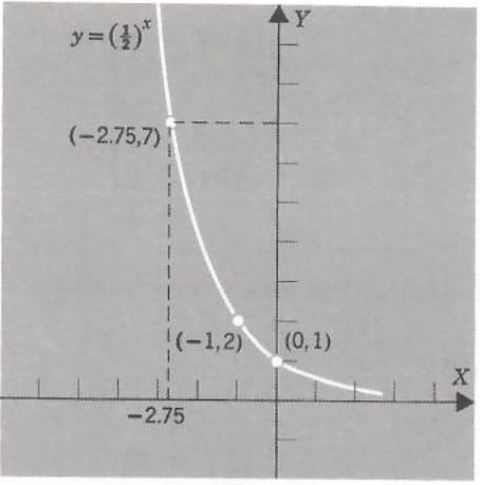
Example 4. Graph y=(1/2)^x
| x | y |
| -3 | (1/2)^(-3)=2^3=8 |
| -2 | (1/2)^(-2)=2^2=4 |
| -3/2 | (1/2)^(-3/2)=2root(2)≈2.8 |
| -1 | (1/2)^(-1)=2 |
| -1/2 | (1/2)^(-1/2)=root(2)≈1.4 |
| 0 | (1/2)^0=1 |
| 1/2 | (1/2)^(1/2)=1/(root(2))=(root(2))/2≈0.7 |
| 1 | (1/2)^1=1/2=0.5 |
| 3/2 | (1/2)^(3/2)=1/(2root(2))=(root(2))/(4)≈0.4 |
| 2 | (1/2)^2=1/4=0.25 |
| 3 | (1/2)^2=1/8≈0.1 |
As in Example 1, it seems reasonable that each horizontal line through a point on the positive y axis intersects the graph of y = (1/2)^x in exactly one point.
Example 5. Estimate (1/2)^(-root(2)) and (1/2)^(root(3)).
First we draw the graph of y = (1/2)^x (see Figure 4)
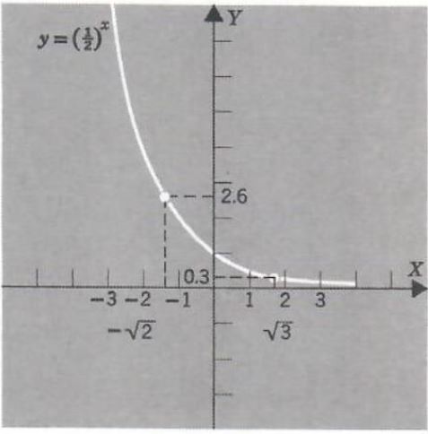
From the graph we have
(1/2)^(-root(2))≈(1/2)^(-1/4)
≈2.6
(1/2)^(root(3))≈(1/2)^(1.7)
≈0.3
Example 6. Solve each of the following equations (a) (1/2)^x=32 (b) (1/2)^x=1/(2root(2)) (c) (1/2)^x=7
(a) Since 2^5=32,
(1/2)^x=32
=2^5
=(1/2)^(-5)
Thus,
x=-5
(b) Since 1/(2root(2))=1/(2*2^(1/2)),
(1/2)^x=1/(2root(2))
=1/(2*2^(1/2))
=1/(2^(3/2))
=(1/2)^(3/2)
Thus,
x=3/2
(c) Since 7 cannot be written as 1/2 to a rational exponent, we use the graph of y = (1/2)^x to estimate x. (See Figure 5.)
From the graph we have
x≈ -2.75
In general, if b is any real number and b>1, then the graph of y=b^x is similar to the graph of y = 2^x. That is, the graph rises as x increases. If b is between 0 and 1, the graph of y = b^x is similar to the graph of y = (1/2)^x, that is, the graph falls as x increases. In both cases each horizontal line through a point on the positive y axis intersects
the graph of y = b^x, (b != 1) in exactly one point. This gives us the
basic property;
P. If b is any positive real number, (b != 1), and a is any positive real number, then there is exactly one real number x such that
b^x=a
This number x is called the logarithm of a to the base b and is denoted by log_(b)a, hence.
b^(log_(b)a)=a
The reason that b = 1 is excluded is that 1^x=1 for all x, so that the graph of y = 1^x is the horizontal straight line through (0, 1). This graph clearly does not satisfy property P. For the rest of this chapter, unless otherwise specified, in either of the expressions b^x or log_(b)x, b is assumed to he positive and different from 1.
It is shown in more advanced texts, that the laws of exponents from Chapter 5 hold for all real exponents. If a and b are positive real numbers, then for all real numbers x and y:
E.1 a^xa^y=a^(x+y)
E.2 (a^x)^y=a^(xy)
E.3 (ab)^x=a^(x)b^(x)
E.4 (a/b)^x=(a^x)/(b^x)
E.5 (a^x)/(a^y)=a^(x-y)
10.2 Logarithmic Functions
From Section 10.1 we recall that for a and b positive, b != 1, the solution to the equitation b^x=a is the real number denoted by log_(b)a. Thus the following two equations are equivalent:
b^x=a
log_(b)a=x
Example 1. Change each of the following equations to its equivalent logarithmic form: (a) 2^3=8 (b) 81^(-1/4)=1/3 (c) 10^x=3
(a) 2^3=8 log_(2)8=3
(b) 81^(-1/4)=1/3 log_(81)(1/3)=-1/4
(c) 10^x=3 log_(10)3=x
Example 2. Change each of the following equations to its equivalent exponential form: (a) log_(3)(9)=2 (b) log_(3/2)(27/8)=3 (c) log_(4)root(2)=1/4 (d) log_(10)3=x
(a) log_3(9)=2 3^2=9
(b) log_(3/2)(27/8)=3 (3/2)^3=27/8
(c) log_4root(2)=1/4 4^(1/4)=root(2)
(d) log_(10)3=x 10^x=3
Example 3. Solve each of the following equations: (a) log_(3)27=x (b) log_(2)x=4 (c) log_(x)64=3
(a) log_(3)27=x
3^x=27
3^x=3^3
x=3
(b) log_(2)x=4
2^4=x
x=16
(c) log_(x)64=3
x^3=64
x^3=4^3
x=4
For all positive real numbers x, the equation
y=log_(b)x
defines y as a function of x. In order to graph this function we use its equivalent exponential equation:
b^y=x
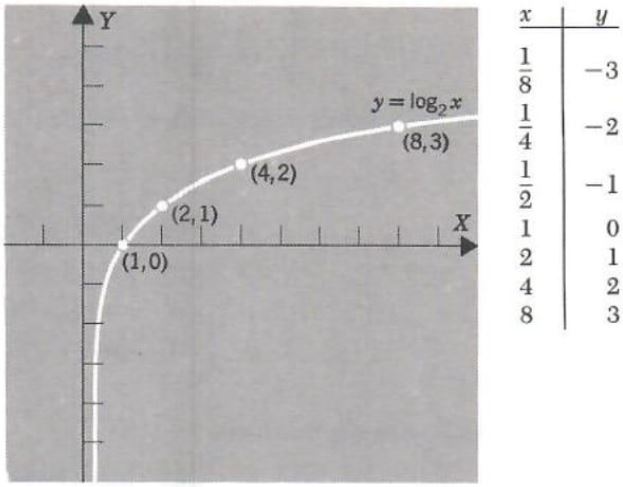
Example 4. Graph y=log_(2)x
The equivalent exponential equation is x=2^y. Points on the graph of this equation are found by choosing values for y and computing the corresponding values for x.
Example 5. Estimate each of the following: (a) log_(2)3 (b) log_(2) (5.6)
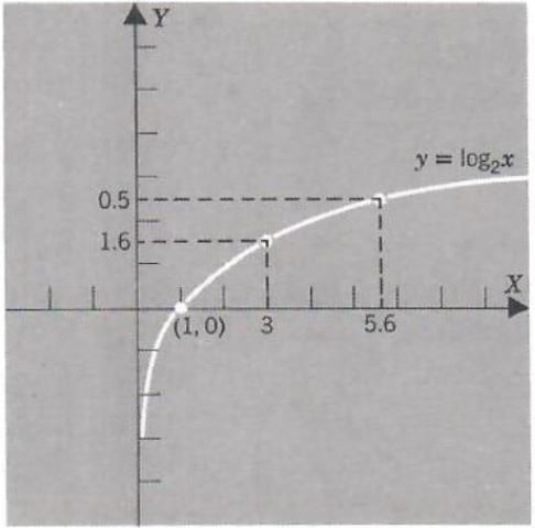
From the graph of y = log_(2)x we have
(a) log_(2)3≈1.6
(b) log_2(5.6)≈2.5
10.3 Properties of Logarithms
From the laws of exponents in Section 9.1, the basic properties of logarithms below are easily derived. For positive real numbers x,y. and b!=1, and real number p:
L.1 log_b(xy)=log_(b)x+log_(b)y
L.2 Log_b(x/y)=log_(b)x-log_(b)y
L.3 log_b(x)^p=(p)log_(b)x
We prove L.1, leaving L.2 and L.3 as exercises. Let
r=log_(b)x and s=log_(b)y
Then,
b^r=x and b^8=y
Therefore,
xy=b^(r)b^(8)
=b^(r+s)
that is,
log_(b)xy=r+s
=log_(b)x+log_(b)y
We will illustrate the use of properties L.1-L.3 in two examples
Example 1. Write 2log_(10)x-1/2log_(10)y+3log_(10)z as a single logarithm.
2log_(10)x-1/2log_(10)y+3log_(10)z
=log_(10)x^2-log_(10)y^(1/2)+log_(10)z^3 (L.3)
=log_(10)x^2z^3-log_(10)y^(1/2) (L.1)
=log_(10)((x^2z^3)/(y^(1/2))) (L.2)
Example 1. Express log_(10)(root(5,(x^2y^3)/(z^4)) as sums and differences of logarithms of the variables.
log_(10)([root(5,(x^2y^3)/(z^4))]
=log_(10)[((x^2y^3)/(x^4))^(1/5)
=1/5log_(10)((x^2y^3)/(x^4)) (L.3)
=1/5[log_(10)x^2+log_(10)y^3-log_(10)z^4 (L.1,L.2)
=2/5log_(10)x+3/5log_(10)y-4/5log_(10)z (L.3)
10.4 Computations with Logarithms
The above laws of logarithms allow us to perform computations that we would normally find quite difficult. We use base 10 logarithms because our number system is written in terms of powers of 10. Using scientific notation we may write every positive real number in the form
n_1.n_2n_3......*10^c
where n_1,n_2,... are integers between 0 and 9 inclusive, n!=0, and c is an integer. Since the tables that we will be using are accurate to three figures, we will round the number off to three significant figures, so that we may write it in the form
(1) n_1.n_2n_3*10^c
In representing a real number A by a decimal expansion we are forced to stop writing digits after only a finite number have been written. That is, we can only use a finite decimal approximation for A. The unwritten digits are said to be rounded off, and the number of digits written, counting from the first nonzero digit on the left to the last digit on the right which is part of the decimal expansion of A, are referred to as significant digits in the given finite decimal approximation for A. For example, the significant digits in 590.61 and 0.00059061 are the same, namely, 5, 9, 0, 6, and 1. However, in 5,906,100 there is some ambiguity. We must find out from the context in which this number appears whether none, one, or both of the last two zeros are significant digits. Thus there may be 5, 6, or 7 significant digits given by 5,906, 100.
Example 1. Write each of the numbers 3,875,262, 0.00076548, 0.008865, and 23150 in form (1)
3,875,262 ≈ 3.88*10^6
0.00076548≈ 7.65*10^-4
0.008865≈ 8.86*10^-3
23150≈ 2.32*10^4
Note that in the last two approximations, if the fourth significant figure is 5 which is followed by zeros only, then we round up if the preceding figure is odd and leave it the same if it is even.
From (1) it follows that if we know the logarithms of numbers between 1 and 10, then we are easily able to find the logarithm of any number. It is common practice to use “=” instead of “≈” in numerical computations. For the remainder of this chapter we will adopt this convention.
Example 2. Express the logarithm to the base 10 of each of the following in terms of a logarithm of a number between 1 and 10: (a) 3,875,262 (b) 00076548.
(a) log_(10)(3,875,262)
=log_(10)(3.88*10^6)
=log_(10)(3.88)+log_(10)(10^6)
=log_(10)(3.88)+6log_(10)(10)
=log_(10)(3.88)+6(1)
=6+log_(10)(3.88)
(b) log_(10)(0.00076548)
=log_(10)(7.65*10^-4)
=log_(10)(7.65)+log_(10)(10^-4)
=log_(10)(7.65)+(-4)log_(10)10
=-4+log_(10)(7.65)
The logarithms to the base 10 of all numbers between 1 and 10 (to two decimal places) are given in Table B on p. 293. We use this table to find log_(10)(3.88) and log_(10)(7.65) in Example 2. To find log_(10)(3.88)
we look in the first column until we find 38, and then find the number in that row which is in the column headed by 8. We find 5888. Since log_10(1) = 0, while log_10(10) = 0, and log_10(3.88) is some real number in-between, we have
log_10(3.88)=0.5888
For the same reason every number in the table is a number between 0 and 1.
In order to find log_10(7.65) we look in the first column to find 76 and then find the number in that row which is in the column headed by 5. We find 8837 and, therefore,
log_10(7.65)=0.8837
From Example 2 we see that
log_10(3,875,262)
= log_(10)(3.88*10^6)
=log_(10)(3.88)+log_(10)(10^6)
=6+log_(10)(3.88)
=6+0.5888
and that
log_(10)(0.00076548)
=log_(10)(7.65*10^-4)
=-4+log_(10)(7.65)
=-4+0.8837
As in Example 2, we see that when a number x is written in form (1),
that is,
x=n_1.n_2n_3*10^c
then
log_10(x)=c+log_10(n_1*n_2n_3)
The integer c is called the characteristic of x and the number log_10(n_1*n_2n_3), which we can find in Table B is called the mantissa of x. Thus the logarithm of a number x is the sum of the characteristic of x and the mantissa. of x. On the other hand, if y is the logarithm of a number x, then x is called the antilog of y.
Example 3. Find the antilog of each of the following: (a) 3.9745 (b) -2+(0.7193) (c) -2.6946.
(a) Since 3.9745=3+0.9745, the integer 3 is the characteristic and 0.9745 is the mantissa. Locate 9745 in Table B. It is in the row headed by 94 and the column headed by 3, so that
log_(10)9.43=0.9745
We have
log_10(x)=3+0.9745
=log_10(10^3)+log_10(9.43)
=log_10(9.43*10^3)
Thus,
x=9.43*10^3
We see that x is in the form of (1) above, where 9.43 is the antilog of the mantissa 0.9745, and the exponent of 10 is the characteristic 3.
(b) The characteristic of -2+0.7193 is -2 , while the mantissa is 0.7193. From Table B,
log_10(5.24)=0.7193
We have
log_10(x)=-2+0.7193
=log_10(5.24-10^-2)
Thus,
x=5.24*10^-2
(c) All the entries in Table B are positive numbers between 0 and 1. Therefore, to use the table we must always express the logarithm of a number as an integer plus a number between 0 and 1. For -2.6946 we find the integer n such that n-2.6946 is a positive number between 0 and 1. Clearly n = 3 is the integer we want. Thus,
-2.6946=-3+3-2.6946
=-3+0.3054
We have
log_10(x)=-2.6946
=-3+0.3054
=-3+log_10(2.02)
=log_10(2.02*10^-3)
Thus,
x=2.02*10^-3
Logarithms are useful in performing computations that involve multiplication, division, and powers (including the extraction of roots). We illustrate with some examples.
Example 4. Calculate ((0.000345)(9,750,000))/((0.0000128))
log_10[((0.000345)(9,750,000))/((0.0000128))
=log_10[((3.45*10^-4)(9.75*10^6))/((1.28*10^-5))
=log_10(3.45*10^-4)+log_10(9.75*10^6)-log_10(1.28*10^-5)
=-4+log_10(3.45)+6+log_10(9.75)-[-5log_10(1.28)
From Table B.
log_10[((0.000345)(9,750,000))/((0.0000128))
=-4+(0.5378)+6+(0.9890)+5-(0.1072)
=7+(1.4196)
=8+0.4196
From Table B, the antilog of 0.4196 is between 2.62, whose logarithm is 0.4183, and 2.63, whose logarithm is 0.4200. In this section we will follow the rule that if the logarithm is halfway or more between the two table entries we will take the larger number for the antilog; otherwise we will take the smaller. Consequently,
log_10[((0.000345)(9,750,000))/((0.0000128))
=8+0.4196
=log_10(10^8)+log_10(2.63)
=log_10(2.63*10^8)
Thus,
((0.000345)(9,750,000))/((0.0000128)) = 2.63*10^8
Example 5. Calculate root(3,0.0000792)(20.9)^(5.31).
log_10root(3,0.0000792)(20.9)^(5.31)
=log_10(7.92*10^-5)^(1/3)+log_10(2.09*10)^(5.31)
=1/3(log_10(7.92)-5)+5.31(log_10(2.09+1)
=1/3(0.8987-5)+5.31(0.3201+1)
=1/3(-4.1013)+5.31(1.3201)
=-1.3671+7.0097
=5.6426
=log_10(4.39x10^5)
Thus,
root(3,0.0000792)(20.9)^(5.31)=4.39*10^5
Example 6. Calculate (root(0.02142))/((4.0325)^(1/4)).
log_10[(root(0.02142))/((4.0325)^(1/4))
=log_10[(2.14*10^-2)^(1/2)]-log_10[(4.0325)^(1.4)
=1/2[-2+log_10(2.14)]-(1.4)log_10(4.03)
=1/2[-2+(0.3304)]-1.4(0.6053)
=1/2(-1.6696)-0.8474
=-0.8348-0.8474
=-1.6822
=-2+2-1.6822
=-2+0.3178
=log_10(10^-2)+log_10(2.08)
Thus,
(root(0.02142))/((4.0325)^(1/4))=2.08*10^-2
10.5 Linear Interpolation
In the last section when the mantissa of a number A was between two entries in the table we approximated A with the antilog of the closest entry. Using the method called linear interpolation we can approximate A to one more decimal place.
Consider the problem of finding the real number A such that
log_10A=0.4197
From table B we have
log_10(2.62)<log_10A<log_10(2.63)
that is,
0.4183<0.4197<0.4200
Consequently,
2.62<A<2.63
Assuming that A divides the interval from 2.62 to 2.63 into the same proportions as its logarithm, 0.4197, divides the interval between the other logarithms, namely, 0.4183 to 0.4200, we obtain the approximation
(A-2.62)/(2.63-2.62)=(0.4197-0.4183)/(0.4200-0.4183)
This approximation can easily be solved for A, adding one more decimal place to the decimal expansion of A.
(A-2.62)/(0.01)=(0.0014)/(0.0017)
A=2.62+14/17*10^-2
A=2.62+0.8*10^-2
A=2.62+0.008
A=2.628
In general, if we have computed log_10X and find that it lies between log_10C and log_10D in the table, then, although we cannot compute Xexactly, we approximate X by X', where X’ is the solution of the following equation.
(1) ![]()
Here X’ is the unknown and the other quantities are known numbers.
The geometric interpretation of equation (1) is that we approximate the actual logarithmic curve between P: (C, log C) and R: (D, log D) by the straight line segment between P and R. For this reason the method is called linear interpolation. See Figure 6. We may derive the equation (1) above, that X’ satisfies, in a geometric way from Figure 6.

Figure 6.
Using similar triangles we have
(TP)/(QP)=(ST)/(RQ)
or
![]()
In Section 10.4 to find log_10X,X was rounded off to three significant figures, since this allows us to find log_10X as a table entry. When using linear interpolation to find log_10X,X is first rounded to four significant figures.
Consider the problem of finding log“, (5.637). From Table B,
log_10(5.62)=0.7497
log_10(5.64)=0.7505
From (1) we obtain the equation
(5.637-5.63)/(5.64-5.63)=(log_10(5.637-0.7497))/(0.7505-0.7497)
Solving for log_10(5.637) we have
log_10(5.637)
=0.7497+((5.637-5.63)/(5.64-5.63))(0.7505-0.7497)
=0.7497+((0.007)/(0.01))(0.0008)
=0.7497+0.00056
=0.75026
=0.7503
Example 1. Interpolate to find X if log_10X=0.5892.
We arrange the entries from the table so that the differences in equation (1) are easily computed:
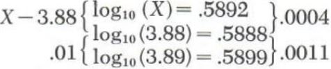
Substituting in equation (1) we have
(X-3.88)/(3.89-3.88)=(log_10X-log_10(3.88))/(log_10(3.89)-log_10(3.88))
=(0.5892-0.5888)/(0.5899-0.5888)
From the diagram above we have
(X-3.88)/(0.01)=(0.0004)/(0.0011)
Solving for X, we obtain
X=3.88+4/11(0.01)
=3.88+0.004
=3.884
Example 1. Interpolate to find log_10(7.924).
From the table we have
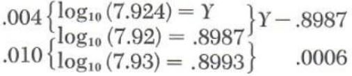
From equation (1) and the diagram,
(0.004)/(0.010)=(Y-0.8987)/(0.0006)
Thus,
log_10(7.924)=Y
=0.8987+4/10(0.0006)
=0.8987+0.0002
=0.8989
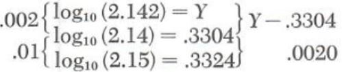
Example 3. Calculate (root(0.02142))/((4.0325)^1.4)
log_10[(root(0.02142))/((4.0325)^1.4)
=log_10[(2.142*10^-2)^(1/2)]-log_10[(4.0325)^1.4
=1/2[-2+log_10(2.142)]-(1.4)log_10(4.032)
Using interpolation we calculate log_10(2.142).
log_10(4.032)=Z
=0.6053+2/10(0.0011)
=0.6055
Thus,
log_10[(root(0.02142))/((4.0325)^1.4)
=1/2[-2+(0.3308)]-(1.4)(0.6055)
=-0.8346-0.8477
=-1.6823
=-2+0.3177
Interpolating we have
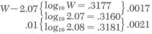
W=2.07+(17)/(21)(0.01)
=2.07+0.008
=2.078
Thus, to four significant figures we have
(root(0.02142))/((4.0325)^1.4)=2.078*10^-2
=0.002078
Compare this with Example 6 of section 10.4.