Description
The plot command will generate a plot of almost any function or relation found in high school and undergraduate college mathematics. It will plot functions given in the form y = f(x), such as y = x2 or y = 3x + 1, as well as relations of the form f(x,y) = g(x,y), such as x2 + y2 = 4.
To use the plot command, simply go to the basic plot page, type in your equation (in terms of x and y), enter the set of x and y values for which the plot should be made and hit the "Plot" button. Your equation will be automatically plotted and the reply will be shown in your browser within a few seconds. If you would like more control over the plotting process, the advanced plot page allows you to show several plots in the one diagram as well as to fine-tune the appearance of the plots with a number of options.
Examples
Here are some examples illustrating the types of equations you can use the plot command on and the results which QuickMath will return.
Basic
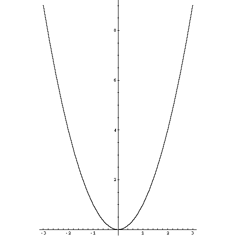
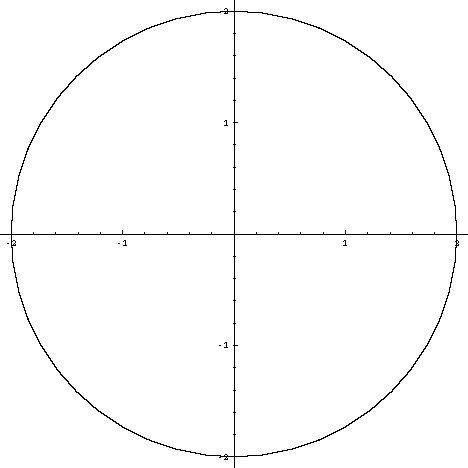
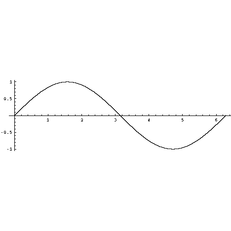
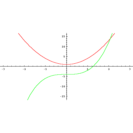
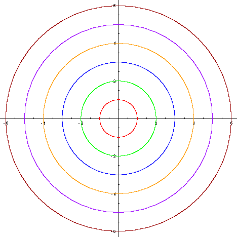
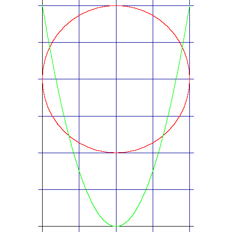
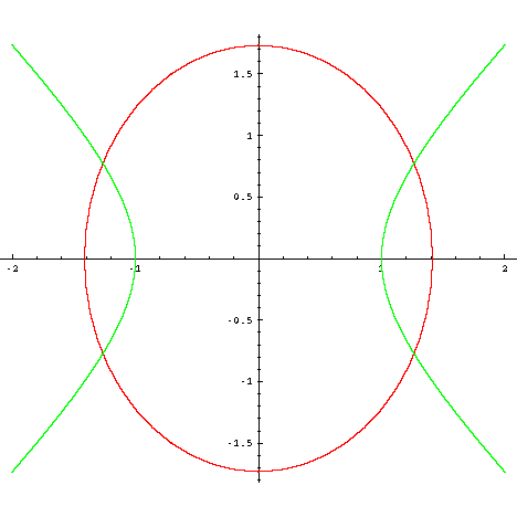
Plot y = 2x + 1 from x = -1 to x = 2 Plot y = x^2 from x = -3 to x = 3 Plot x^2 + y^2 = 4 from x = -2 to x = 2 Plot y = sin(x) from x = 0 to x = 2 pi Plot y = 3x^2 + 1 and y = 2x^3 - 4 from x = -3 to x = 3, y = -17 to y = 17 with an aspect ratio of 1 : 2 Plot x^2 + y^2 = 1, x^2 + y^2 = 4, x^2 + y^2 = 9, x^2 + y^2 =16,x^2 + y^2 = 25 and x^2 + y^2 =36 from x = -6 to x = 6, y = -6 to y = 6 Plot (x-1)^2+(y-2)^2=1 and y=3(x-1)^2 from x = 0 to x = 2, y = 0 to y = 3 showing grid lines, but no tick marks. Plot x^2/2+y^2/3=1 and x^2-y^2=1 from x = -2 to x = 2, y = -1.8 to y = 1.8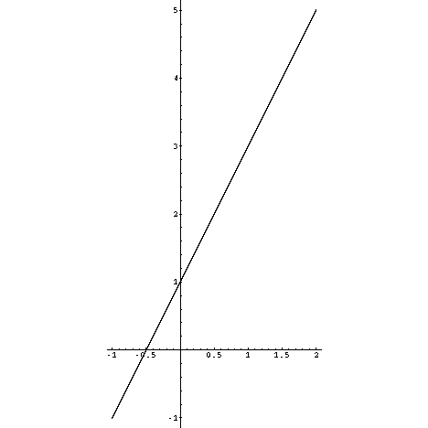
Options (advanced page only)
Tick marksValues : checked or unchecked
Default : checked
When Tick marks is checked, the axes on the plot will show tick marks and numerical scales.
Grid lines
Values : checked or unchecked
Default : unchecked
When Grid lines is checked, a blue grid will be superimposed on the graph.
Axes
Values : None or Automatic origin or Origin at (#,#)
Default : Automatic origin
The Axes option controls the appearance and location of the axes on the plot. When None is checked, no axes will be shown at all. When Automatic origin is checked, axes will be shown. The two axes will usually intersect at (0,0), but sometimes this point of intersection will be located elsewhere. When Origin at (#,#) is checked and a point is entered, the axes will be shown and their point of intersection will be forced to be at the specified point.
Aspect ratio
Values : One to one or Golden ratio or # : #
Default : One to one
The Aspect ratio option controls the ratio of the height of the plot to its width. When One to one is checked the ratio is 1:1 and the scales on the two axes will be identical. This will ensure that circles, for example, will actually appear circular on the screen. When Golden ratio is selected, the aspect ratio is 1 : 1/g, where g is the Golden Ratio (approximately 1.6180). This supposedly gives a ratio of height to width which is especially 'pleasing' to the eye. When # : # is selected and two values are entered, the specified aspect ratio will be applied. This is useful if the plot is highly compressed in one direction or the other and needs to be 'stretched-out' to make it clearer.