Systems of Equations and Inequalities
In previous chapters we solved equations with one unknown or variable. We will now study methods of solving systems of equations consisting of two equations and two variables.
POINTS ON THE PLANE
OBJECTIVES
Upon completing this section you should be able to:
- Represent the Cartesian coordinate system and identify the origin and axes.
- Given an ordered pair, locate that point on the Cartesian coordinate system.
- Given a point on the Cartesian coordinate system, state the ordered pair associated with it.
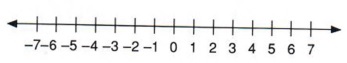
We have already used the number line on which we have represented numbers as points on a line.
Note that this concept contains elements from two fields of mathematics, the line from geometry and the numbers from algebra. Rene Descartes (1596-1650) devised a method of relating points on a plane to algebraic numbers. This scheme is called the Cartesian coordinate system (for Descartes) and is sometimes referred to as the rectangular coordinate system.
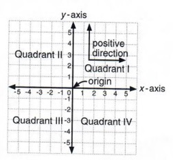
This system is composed of two number lines that are perpendicular at their zero points.
| Perpendicular means that two lines are at right angles to each other. |
Study the diagram carefully as you note each of the following facts.
The number lines are called axes. The horizontal line is the x-axis and the vertical is the y-axis. The zero point at which they are perpendicular is called the origin.
| Axes is plural. Axis is singular. |
Positive is to the right and up; negative is to the left and down.
| The arrows indicate the number lines extend indefinitely. Thus the plane extends indefinitely in all directions. |
The plane is divided into four parts called quadrants. These are numbered in a counterclockwise direction starting at the upper right.
Points on the plane are designated by ordered pairs of numbers written in parentheses with a comma between them, such as (5,7). This is called an ordered pair because the order in which the numbers are written is important. The ordered pair (5,7) is not the same as the ordered pair (7,5). Points are located on the plane in the following manner.
First, start at the origin and count left or right the number of spaces designated by the first number of the ordered pair. Second, from the point on the x-axis given by the first number count up or down the number of spaces designated by the second number of the ordered pair. Ordered pairs are always written with x first and then y, (x,y). The numbers represented by x and y are called the coordinates of the point (x,y).
| This is important. The first number of the ordered pair always refers to the horizontal direction and the second number always refers to the vertical direction. |
Example 1 On the following Cartesian coordinate system the points A (3,4), B (0,5), C (-2,7), D (-4,1), E (-3,-4), F (4,-2), G (0,-5), and H (-6,0) are designated. Check each one to determine how they are located.
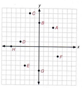
| What are the coordinates of the origin? |
GRAPHING LINEAR EQUATIONS
OBJECTIVES
Upon completing this section you should be able to:
- Find several ordered pairs that make a given linear equation true.
- Locate these points on the Cartesian coordinate system.
- Draw a straight line through those points that represent the graph of this equation.
A graph is a pictorial representation of numbered facts. There are many types of graphs, such as bar graphs, circular graphs, line graphs, and so on. You can usually find examples of these graphs in the financial section of a newspaper. Graphs are used because a picture usually makes the number facts more easily understood.
In this section we will discuss the method of graphing an equation in two variables. In other words, we will sketch a picture of an equation in two variables.
Consider the equation x + y - 7 and note that we can easily find many solutions. For instance, if x = 5 then y - 2, since 5 + 2 = 7. Also, if x = 3 then y = 4, since 3 + 4 = 7. If we represent these answers as ordered pairs (x,y), then we have (5,2) and (3,4) as two points on the plane that represent answers to the equation x + y = 7.
All possible answers to this equation, located as points on the plane, will give us the graph (or picture) of the equation.
Of course we could never find all numbers x and y such that x + y = 7, so we must be content with a sketch of the graph. A sketch can be described as the "curve of best fit." In other words, it is necessary to locate enough points to give a reasonably accurate picture of the equation.
| Remember, there are infinitely many ordered pairs that would satisfy the equation. |
Example 1 Sketch the graph of 2x + y = 3.
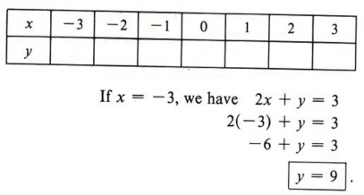
Solution We wish to find several pairs of numbers that will make this equation true. We will accomplish this by choosing a number for x and then finding a corresponding value for y. A table of values is used to record the data.
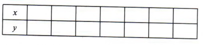
In the top line (x) we will place numbers that we have chosen for x. Then in the bottom line (y) we will place the corresponding value of y derived from the equation.
| Of course, we could also start by choosing values for y and then find the corresponding values for x. |
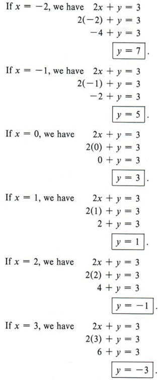
In this example we will allow x to take on the values -3, -2, -1,0, 1,2,3.
| These values are arbitrary. We could choose any values at all. |
| Notice that once we have chosen a value for x, the value for y is determined by using the equation. |
These values of x give integers for values of y. Thus they are good choices. Suppose we chose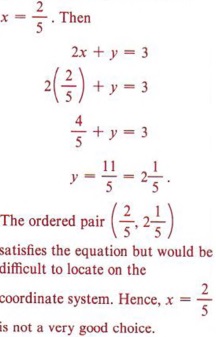 |
These facts give us the following table of values:
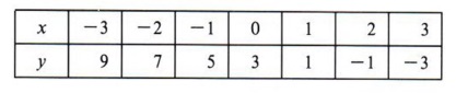
We now locate the ordered pairs (-3,9), (-2,7), (-1,5), (0,3), (1,1), (2,-1), (3,-3) on the coordinate plane and connect them with a line.
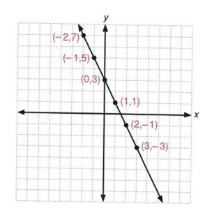
We now have the graph of 2x + y = 3.
| The line indicates that all points on the line satisfy the equation, as well as the points from the table. The arrows indicate the line continues indefinitely. |
The graphs of all first-degree equations in two variables will be straight lines. This fact will be used here even though it will be much later in mathematics before you can prove this statement. Such first-degree equations are called linear equations.
| Thus, any equation of the form ax + by - c where a, b, and c are real numbers is a linear equation. |
Equations in two unknowns that are of higher degree give graphs that are curves of different kinds. You will study these in future algebra courses.
Since the graph of a first-degree equation in two variables is a straight line, it is only necessary to have two points. However, your work will be more consistently accurate if you find at least three points. Mistakes can be located and corrected when the points found do not lie on a line. We thus refer to the third point as a "checkpoint."
| This is important. Don't try to shorten your work by finding only two points. You will be surprised how often you will find an error by locating all three points. |
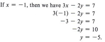
Example 2 Sketch the graph of 3x - 2y - 7.
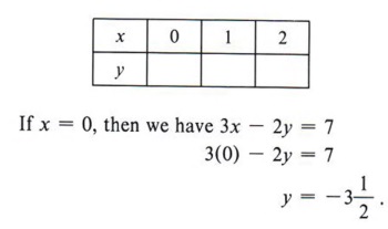
Solution First make a table of values and decide on three numbers to substitute for x. We will try 0, 1,2.
| Again, you could also have started with arbitrary values of y. |
The answer ![]() is not as easy to locate on the graph as an integer would be. So it seems that x = 0 was not a very good choice. Sometimes it is possible to look ahead and make better choices for x.
is not as easy to locate on the graph as an integer would be. So it seems that x = 0 was not a very good choice. Sometimes it is possible to look ahead and make better choices for x.
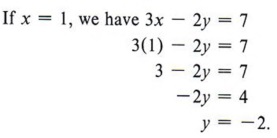
| Since both x and y are integers, x = 1 was a good choice. |
The point (1,-2) will be easier to locate. If x = 2, we will have another fraction.
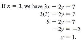
The point (3,1) will be easy to locate.
| x = 3 was another good choice. |
We will readjust the table of values and use the points that gave integers. This may not always be feasible, but trying for integral values will give a more accurate sketch. We now have the table for 3x - 2y = 7.
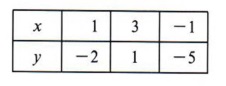
| We can do this since the choices for x were arbitrary. |
Locating the points (1,-2), (3,1), (- 1,-5) gives the graph of 3x - 2y = 7.
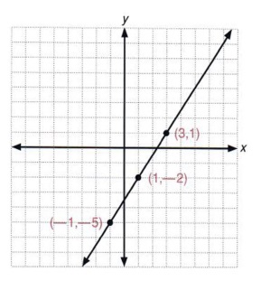
| How many ordered pairs satisfy this equation? |
SLOPE OF A LINE
OBJECTIVES
Upon completing this section you should be able to:
- Associate the slope of a line with its steepness.
- Write the equation of a line in slope-intercept form.
- Graph a straight line using its slope and y-intercept.
We now wish to discuss an important concept called the slope of a line. Intuitively we can think of slope as the steepness of the line in relationship to the horizontal.
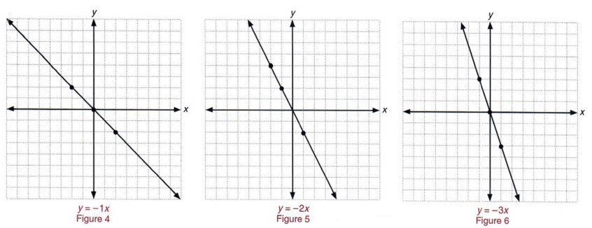
Following are graphs of several lines. Study them closely and mentally answer the questions that follow.
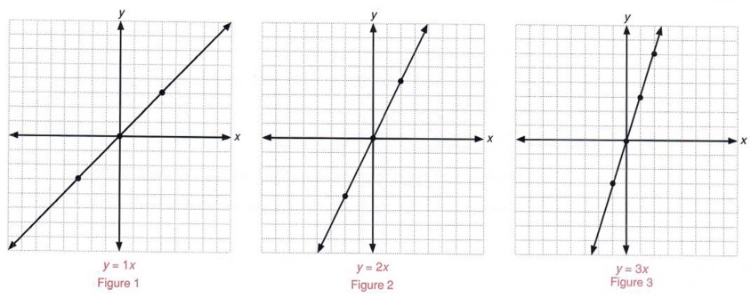
Which line is steeper?
What seems to be the relationship between the coefficient of x and the steepness Which graph would be steeper: of the line when the equation is of the form y = mx?
| Which graph would be steeper: y = 3x or y = 7x? |
Now study the following graphs.
Which line is steeper?
What effect does a negative value for m have on the graph?
| Which graph would be steeper: y = 3x or y = 7x? |
For the graph of y = mx, the following observations should have been made.
- If m > 0, then
- as the value of m increases, the steepness of the line increases and
- the line rises to the right and falls to the left.
- If m < 0, then
- as the value of m increases, the steepness of the line decreases and
- the line rises to the left and falls to the right
| Remember, m > 0 means "m is greater than zero." |
In other words, in an equation of the form y - mx, m controls the steepness of the line. In mathematics we use the word slope in referring to steepness and form the following definition:
In an equation of the form y = mx, m is the slope of the graph of the equation.
Example 1 Sketch the graph of y = 6x and give the slope of the line.
Solution We first make a table showing three sets of ordered pairs that satisfy the equation.
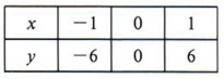
| Remember, we only need two points to determine the line but we use the third point as a check. |
We then sketch the graph.
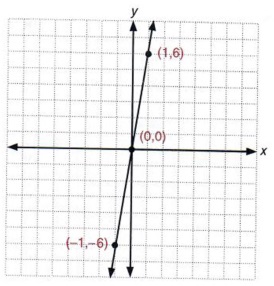
The value of m is 6, therefore the slope is 6. We may merely write m - 6.

Example 2 Sketch the graph and state the slope of 
Solution Choosing values of x that are divisible by 3, we obtain the table
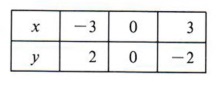
| Why use values that are divisible by 3? |
Then the graph is
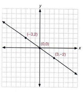
The slope of 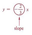
We now wish to compare the graphs of two equations to establish another concept.
Example 3 Sketch the graphs of y 3x and y - 3x + 2 on the same set of coordinate axes.
| Compare the coefficients of x in these two equations. |
Solution 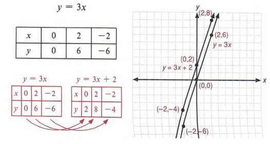
In example 3 look at the tables of values and note that for a given value of x, the value of y in the equation y = 3x + 2 is two more than the corresponding value of y in the equation y = 3x.
Look now at the graphs of the two equations and note that the graph of y = 3x + 2 seems to have the same slope as y = 3x. Also note that if the entire graph of y = 3x is moved upward two units, it will be identical with the graph of y = 3x + 2. The graph of y = 3x crosses the y-axis at the point (0,0), while the graph of y = 3x + 2 crosses the y-axis at the point (0,2).
| Again, compare the coefficients of x in the two equations. |
Compare these tables and graphs as in example 3.
| Observe that when two lines have the same slope, they are parallel. |
The slope from one point on a line to another is determined by the ratio of the change in y to the change in x. That is,
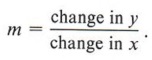
| If you want to impress your friends, you can write where the Greek letter |
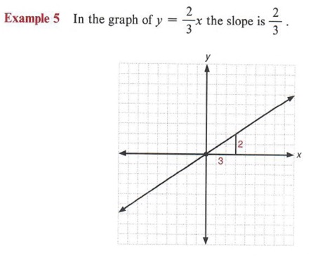
Note that the change in x is 3 and the change in y is 2.
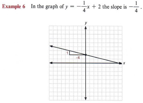
The change in x is -4 and the change in y is 1.
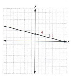 We could also say that the change in x is 4 and the change in y is - 1. This will result in the same line. |
Example 7 In the graph of y = 3x - 2 the slope is 3.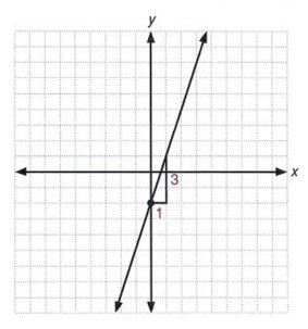
The change in x is 1 and the change in y is 3.
y = mx + b is called the slope-intercept form of the equation of a straight line. If an equation is in this form, m is the slope of the line and (0,b) is the point at which the graph intercepts (crosses) the y-axis.
| The point (0,b) is referred to as the y-intercept. |
If the equation of a straight line is in the slope-intercept form, it is possible to sketch its graph without making a table of values. Use the y-intercept and the slope to draw the graph, as shown in example 8.
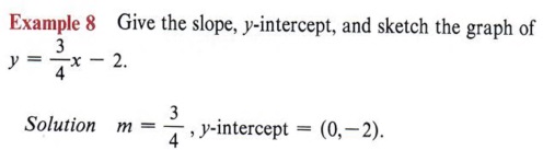
| Note that this equation is in the form y = mx + b. |
First locate the point (0,-2). This is one of the points on the line. The slope indicates that the changes in x is 4, so from the point (0,-2) we move four units in the positive direction parallel to the x-axis. Since the change in y is 3, we then move three units in the positive direction parallel to the y-axis. The resulting point is also on the line. Since two points determine a straight line, we then draw the graph.
| Always start from the y-intercept. A common error that many students make is to confuse the y-intercept with the x-intercept (the point where the line crosses the x-axis). |
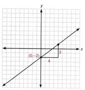
Example 9 Give the slope and y-intercept and sketch the graph of y = 3x + 4.
Solution m = -3, y-intercept = (0,4).
To express the slope as a ratio we may write -3 as ![]() or
or ![]() . If we write the slope as
. If we write the slope as ![]() , then from the point (0,4) we move one unit in the positive direction parallel to the x-axis and then move three units in the negative direction parallel to the y-axis. Then we draw a line through this point and (0,4).
, then from the point (0,4) we move one unit in the positive direction parallel to the x-axis and then move three units in the negative direction parallel to the y-axis. Then we draw a line through this point and (0,4).
Suppose an equation is not in the form y = mx + b. Can we still find the slope and y-intercept? The answer to this question is yes. To do this, however, we must change the form of the given equation by applying the methods used in section 4-2.
| Section 4-2 dealt with solving literal equations. You may want to review that section. |
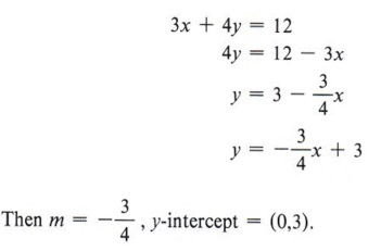
Example 10 Find the slope and y-intercept of 3x + 4y = 12.
Solution First we recognize that the equation is not in the slope-intercept form needed to answer the questions asked. To obtain this form solve the given equation for y.
 Sketch the graph of Sketch the graph of |
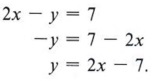
Example 11 Find the slope and y-intercept of 2x - y = 7.
Solution Placing the equation in slope-intercept form, we obtain
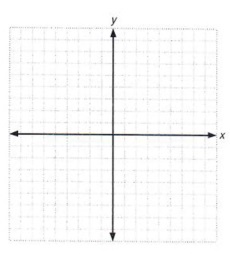
| Sketch the graph of the line on the grid below. |
GRAPHING LINEAR INEQUALITIES
OBJECTIVES
Upon completing this section you should be able to graph linear inequalities.
In chapter 4 we constructed line graphs of inequalities such as
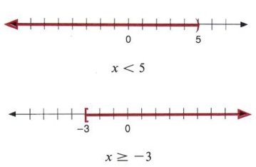
These were inequalities involving only one variable. We found that in all such cases the graph was some portion of the number line. Since an equation in two variables gives a graph on the plane, it seems reasonable to assume that an inequality in two variables would graph as some portion or region of the plane. This is in fact the case. The solution of the inequality x + y < 5 is the set of all ordered pairs of numbers {x,y) such that their sum is less than 5. (x + y < 5 is a linear inequality since x + y = 5 is a linear equation.)
Example 1 Are each of the following pairs of numbers in the solution set of x + y < 5? (2,1), (3,-4), (5,6), (3,2), (0,0), (-1,4), (-2,8).
Solution
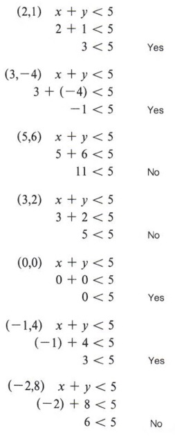
| The solution set consists of all ordered pairs that make the statement true. |
| To summarize, the following ordered pairs give a true statement. (2,1),(3,-4),(0,0),(-1,4) |
| The following ordered pairs give a false statement. (5,6),(3,2),(-2,8) |
Following is a graph of the line x + y = 5. The points from example 1 are indicated on the graph with answers to the question "Is x + y < 5?"
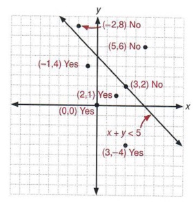
| Notice that all the points that satisfy the equation are to the left and below the line while all the points that will not are above and to the right. |
Observe that all "yes" answers lie on the same side of the line x + y = 5, and all "no" answers lie on the other side of the line or on the line itself.
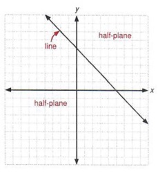
The graph of the line x + y = 5 divides the plane into three parts: the line itself and the two sides of the lines (called half-planes).
x + y < 5 is a half-plane
x + y < 5 is a line and a half-plane.
If one point of a half-plane is in the solution set of a linear inequality, then all points in that half-plane are in the solution set. This gives us a convenient method for graphing linear inequalities.
To graph a linear inequality
1. Replace the inequality symbol with an equal sign and graph the resulting line.
2. Check one point that is obviously in a particular half-plane of that line to see if it is in the solution set of the inequality.
3. If the point chosen is in the solution set, then that entire half-plane is the solution set. If the point chosen is not in the solution set, then the other half-plane is the solution set.
| Why do we need to check only one point? |
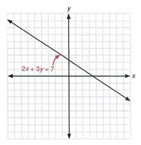
Example 2 Sketch the graph of 2x 4- 3y > 7.
Solution Step 1: First sketch the graph of the line 2x + 3y = 7 using a table of values or the slope-intercept form.
Step 2: Next choose a point that is not on the line 2x + 3y = 7. [If the line does not go through the origin, then the point (0,0) is always a good choice.] Now turn to the inequality 2x + 3y> > 7 to see if the chosen point is in the solution set.
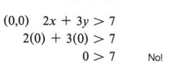
Step 3: The point (0,0) is not in the solution set, therefore the half-plane containing (0,0) is not the solution set. Hence, the other halfplane determined by the line 2x + 3y = 7 is the solution set.
Since the line itself is not a part of the solution, it is shown as a dashed line and the half-plane is shaded to show the solution set.
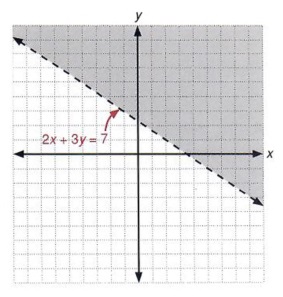
| The solution set is the half-plane above and to the right of the line. |
Example 3 Graph the solution for the linear inequality 2x - y ≥ 4.
Solution Step 1: First graph 2x - y = 4. Since the line graph for 2x - y = 4 does not go through the origin (0,0), check that point in the linear inequality.
Step 2: 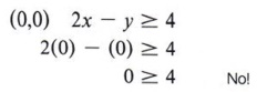
Step 3: Since the point (0,0) is not in the solution set, the half-plane containing (0,0) is not in the set. Hence, the solution is the other half-plane. Notice, however, that the line 2x - y = 4 is included in the solution set. Therefore, draw a solid line to show that it is part of the graph.
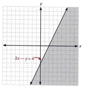
| The solution set is the line and the half-plane below and to the right of the line. |
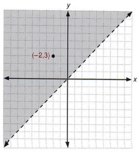
Example 4 Graph x < y.
Solution First graph x = y. Next check a point not on the line. Notice that the graph of the line contains the point (0,0), so we cannot use it as a checkpoint. To determine which half-plane is the solution set use any point that is obviously not on the line x = y. The point ( - 2,3) is such a point.
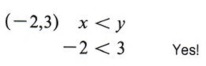
Using this information, graph x < y.
| When the graph of the line goes through the origin, any other point on the x- or y-axis would also be a good choice. |
GRAPHICAL SOLUTION OF A SYSTEM OF LINEAR EQUATIONS
OBJECTIVES
Upon completing this section you should be able to:
- Sketch the graphs of two linear equations on the same coordinate system.
- Determine the common solution of the two graphs.
Example 1 The pair of equations 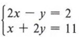 is called a system of linear equations.
We have observed that each of these equations has infinitely many solutions and each will form a straight line when we graph it on the Cartesian coordinate system.
We now wish to find solutions to the system. In other words, we want all points (x,y) that will be on the graph of both equations.
Solution We reason in this manner: If all solutions of 2x - y = 2 lie on one straight line and all solutions of x + 2y = 11 lie on another straight line, then a solution to both equations will be their points of intersection (if the two lines intersect).
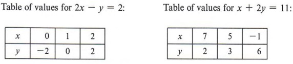
| In this table we let x take on the values 0, 1, and 2. We then find the values for y by using the equation. Do this before going on. In this table we let y take on the values 2, 3, and 6. We then find x by using the equation. Check these values also. |
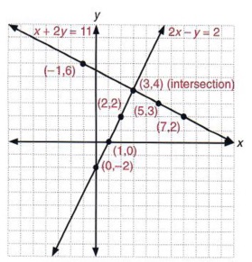
| The two lines intersect at the point (3,4). |
Note that the point of intersection appears to be (3,4). We must now check the point (3,4) in both equations to see that it is a solution to the system.
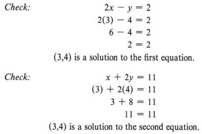
| As a check we substitute the ordered pair (3,4) in each equation to see if we get a true statement. Are there any other points that would satisfy both equations? Why? |
Therefore, (3,4) is a solution to the system.
Not all pairs of equations will give a unique solution, as in this example. There are, in fact, three possibilities and you should be aware of them.
Since we are dealing with equations that graph as straight lines, we can examine these possibilities by observing graphs.
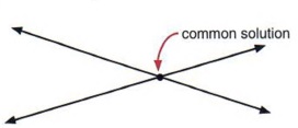
1. Independent equations The two lines intersect in a single point. In this case there is a unique solution.
| The example above was a system of independent equations. |
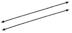
2. Inconsistent equations The two lines are parallel. In this case there is no solution.
| No matter how far these lines are extended, they will never intersect. |
3. Dependent equations The two equations give the same line. In this case any solution of one equation is a solution of the other.
| In this case there will be infinitely many common solutions. |
In later algebra courses, methods of recognizing inconsistent and dependent equations will be learned. However, at this level we will deal only with independent equations. You can then expect that all problems given in this chapter will have unique solutions.
| This means the graphs of all systems in this chapter will intersect in a single point. |
To solve a system of two linear equations by graphing
1. Make a table of values and sketch the graph of each equation on the same coordinate system.
2. Find the values of (x,y) that name the point of intersection of the lines.
3. Check this point (x,y) in both equations.
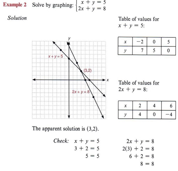
| Again, in this table wc arbitrarily selected the values of x to be - 2, 0, and 5. Here we selected values for x to be 2, 4, and 6. You could have chosen any values you wanted. We say "apparent" because we have not yet checked the ordered pair in both equations. Once it checks it is then definitely the solution. |
Since (3,2) checks in both equations, it is the solution to the system.
GRAPHICAL SOLUTION OF A SYSTEM OF LINEAR INEQUALITIES
OBJECTIVES
Upon completing this section you should be able to:
- Graph two or more linear inequalities on the same set of coordinate axes.
- Determine the region of the plane that is the solution of the system.
Later studies in mathematics will include the topic of linear programming. Even though the topic itself is beyond the scope of this text, one technique used in linear programming is well within your reach-the graphing of systems of linear inequalities-and we will discuss it here.
You found in the previous section that the solution to a system of linear equations is the intersection of the solutions to each of the equations. In the same manner the solution to a system of linear inequalities is the intersection of the half-planes (and perhaps lines) that are solutions to each individual linear inequality.
In other words, x + y > 5 has a solution set and 2x - y < 4 has a solution set. Therefore, the system
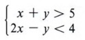
has as its solution set the region of the plane that is in the solution set of both inequalities.
To graph the solution to this system we graph each linear inequality on the same set of coordinate axes and indicate the intersection of the two solution sets.
| Note that the solution to a system of linear inequalities will be a collection of points. |
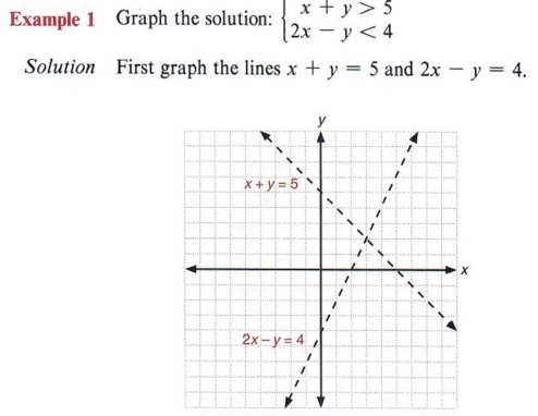
| Again, use either a table of values or the slope-intercept form of the equation to graph the lines. |
Checking the point (0,0) in the inequality x + y > 5 indicates that the point (0,0) is not in its solution set. We indicate the solution set of x + y > 5 with a screen to the right of the dashed line.
| This region is to the right and above the line x + y = 5. |
Checking the point (0,0) in the inequality 2x - y < 4 indicates that the point (0,0) is in its solution set. We indicate this solution set with a screen to the left of the dashed line.
| This region is to the left and above the line 2x - y = 4. |
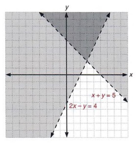
The intersection of the two solution sets is that region of the plane in which the two screens intersect. This region is shown in the graph.
Note again that the solution does not include the lines. If, for example, we were asked to graph the solution of the system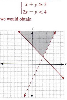 which indicates the solution includes points on the line x+ y = 5. |
The results indicate that all points in the shaded section of the graph would be in the solution sets of x + y > 5 and 2x - y < 4 at the same time.
SOLVING A SYSTEM BY SUBSTITUTION
OBJECTIVES
Upon completing this section you should be able to solve a system of two linear equations by the substitution method.
In section 6-5 we solved a system of two equations with two unknowns by graphing. The graphical method is very useful, but it would not be practical if the solutions were fractions. The actual point of intersection could be very difficult to determine.
There are algebraic methods of solving systems. In this section we will discuss the method of substitution.
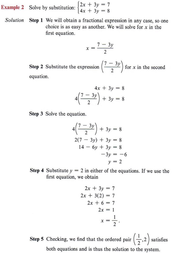
Example 1 Solve by the substitution method: 
Solution
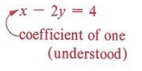
Step 1 We must solve for one unknown in one equation. We can choose either x or y in either the first or second equation. Our choice can be based on obtaining the simplest expression. In this case we will solve for x in the second equation, obtaining x = 4 + 2y, because any other choice would have resulted in a fraction.
| Look at both equations and see if either of them has a variable with a coefficient of one. |
Step 2 Substitute the value of x into the other equation. In this case the equation is
2x + 3y = 1.
Substituting (4 + 2y) for x, we obtain 2(4 + 2y) + 3y = 1, an equation with only one unknown.
| The reason for this is that if x = 4 + 2y in one of the equations, then x must equal 4 + 2y in the other equation. |
Step 3 Solve for the unknown.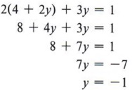
| Remember, first remove parentheses. |
Step 4 Substitute y = - 1 into either equation to find the corresponding value for x. Since we have already solved the second equation for x in terms of y, we may use it.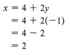
| We may substitute y = - 1 in either equation since y has the same value in both. |
Thus, we have the solution (2,-1).
| Remember, x is written first in the ordered pair. |
Step 5 Check the solution in both equations. Remember that the solution for a system must be true for each equation in the system. Since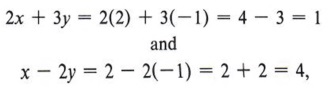
the solution (2,-1) does check.
| This checks: 2x + 3y = 1 and x - 2y = 4. |
| Check this ordered pair in both equations. Neither of these equations had a variable with a coefficient of one. In this case, solving by substitution is not the best method, but we will do it that way just to show it can be done. The next section will give us an easier method. |
SOLVING A SYSTEM OF LINEAR EQUATIONS BY ADDITION
OBJECTIVES
Upon completing this section you should be able to solve a system of two linear equations by the addition method.
The addition method for solving a system of linear equations is based on two facts that we have used previously.
First we know that the solutions to an equation do not change if every term of that equation is multiplied by a nonzero number. Second we know that if we add the same or equal quantities to both sides of an equation, the results are still equal.
Example 1 Solve by addition: 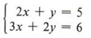
| Note that we could solve this system by the substitution method, by solving the first equation for y. Solve this system by the substitution method and compare your solution with that obtained in this section. |
Solution
Step 1 Our purpose is to add the two equations and eliminate one of the unknowns so that we can solve the resulting equation in one unknown. If we add the equations as they are, we will not eliminate an unknown. This means we must first multiply each side of one or both of the equations by a number or numbers that will lead to the elimination of one of the unknowns when the equations are added.
After carefully looking at the problem, we note that the easiest unknown to eliminate is y. This is done by first multiplying each side of the first equation by -2.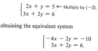
| Note that each term must be multiplied by ( - 2). |
Step 2 Add the equations.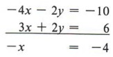
Step 3 Solve the resulting equation.![]()
| In this case we simply multiply each side by (-1). |
Step 4 Find the value of the other unknown by substituting this value into one of the original equations. Using the first equation,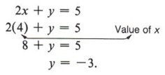
| Substitute x = 4 in the second equation and see if you get the same value for y. |
Step 5 If we check the ordered pair (4,-3) in both equations, we see that it is a solution of the system.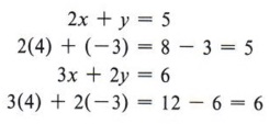
Example 2 Solve by addition: ![]()
| Note that in this system no variable has a coefficient of one. Therefore, the best method of solving it is the addition method. |
Solution
Step 1 Both equations will have to be changed to eliminate one of the unknowns. Neither unknown will be easier than the other, so choose to eliminate either x or y.
To eliminate x multiply each side of the first equation by 3 and each side of the second equation by -2.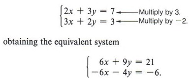
| If you choose to eliminate y, multiply the first equation by - 2 and the second equation by 3. Do this and solve the system. Compare your solution with the one obtained in the example. |
Step 2 Adding the equations, we obtain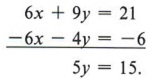
Step 3 Solving for y yields![]()
Step 4 Using the first equation in the original system to find the value of the other unknown gives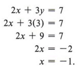
Step 5 Check to see that the ordered pair ( - 1,3) is a solution of the system.
| The check is left up to you. |
STANDARD FORM
OBJECTIVES
Upon completing this section you should be able to:
- Write a linear equation in standard form.
- Solve a system of two linear equations if they are given in nonstandard form.
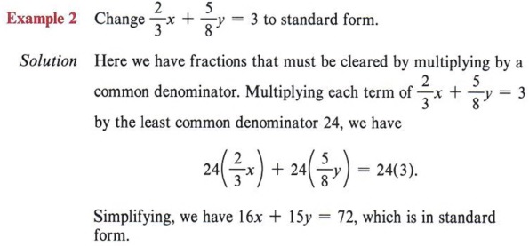
Equations in the preceding sections have all had no fractions, both unknowns on the left of the equation, and unknowns in the same order.
Such equations are said to be in standard form. That is, they are in the form ax + by = c, where a, b and c are integers. Equations must be changed to the standard form before solving by the addition method.
Example 1 Change 3x = 5 + 4y to standard form.
Solution 3x = 5 + 4y is not in standard form because one unknown is on the right. If we add -4y to both sides, we have 3x - 4y = 5, which is in standard form.
| Be careful here. Many students forget to multiply the right side of the equation by 24. |
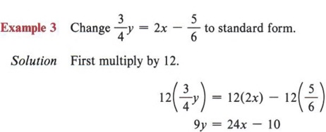
| Again, make sure each term is multiplied by 12. |
Now add - 24x to both sides, giving - 24x + 9y = -10, which is in standard form. Usually, equations are written so the first term is positive. Thus we multiply each term of this equation by (- 1).
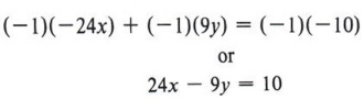
| Instead of saying "the first term is positive," we sometimes say "the leading coefficient is positive." |
WORD PROBLEMS WITH TWO UNKNOWNS
OBJECTIVES
Upon completing this section you should be able to:
- Determine when a word problem can be solved using two unknowns.
- Determine the equations and solve the word problem.
Many word problems can be outlined and worked more easily by using two unknowns.
Example 1 The sum of two numbers is 5. Three times the first number added to five times the second number is 9. Find the numbers.
Solution Let x = first number
y = second number
The first statement gives us the equation
x + y = 5.
The second statement gives us the equation
3x + 5 y = 9.
We now have the system
which we can solve by either method we have learned, to give
x = 8 and y = - 3.
| Solve the system by substitution. |
Example 2 Two workers receive a total of $136 for 8 hours work. If one worker is paid $1.00 per hour more than the other, find the hourly rate for each.
Solution Let x = hourly rate of one worker
y = hourly rate of other worker.
| Note that it is very important to say what x and y represent. |
The first statement gives us the equation
8x + 8y = 136.
The second statement gives the equation
x = y + 1.
We now have the system (in standard form)
Solving gives x = 9 and y = 8. One worker's rate is $9.00 per hour and the other's is $8.00 per hour.
| Solve this system by the addition method. |
SUMMARY
Key Words
- The Cartesian coordinate system is a method of naming points on a plane.
- Ordered pairs of numbers are used to designate points on a plane.
- A linear equation graphs a straight line.
- The slope from one point on a line to another is the ratio
 .
. - The slope-intercept form of the equation of a line is y = mx + b.
- A linear inequality graphs as a portion of the plane.
- A system of two linear equations consists of linear equations for which we wish to find a simultaneous solution.
- Independent equations have unique solutions.
- Inconsistent equations have no solution.
- Dependent equations have infinitely many solutions.
- A system of two linear inequalities consists of linear inequalities for which we wish to find a simultaneous solution.
- The standard form of a linear equation is ax + by = c, where a, b, and c are real numbers.
Procedures
- To sketch the graph of a linear equation find ordered pairs of numbers that are solutions to the equation. Locate these points on the Cartesian coordinate system and connect them with a line.
- To sketch the graph of a line using its slope:
Step 1 Write the equation of the line in the form y - mx + b.
Step 2 Locate the j-intercept (0,b).
Step 3 Starting at (0,b), use the slope m to locate a second point.
Step 4 Connect the two points with a straight line. - To graph a linear inequality:
Step 1 Replace the inequality symbol with an equal sign and graph the resulting line.
Step 2 Check one point that is obviously in a particular half-plane of that line to see if it is in the solution set of the inequality.
Step 3 If the point chosen is in the solution set, then that entire half-plane is the solution set. If the point chosen is not in the solution set, then the other halfplane is the solution set. - To solve a system of two linear equations by graphing, graph the equations carefully on the same coordinate system. Their point of intersection will be the solution of the system.
- To solve a system of two linear inequalities by graphing, determine the region of the plane that satisfies both inequality statements.
- To solve a system of two equations with two unknowns by substitution, solve for one unknown of one equation in terms of the other unknown and substitute this quantity into the other equation. Then substitute the numerical value thus found into either equation to find the value of the other unknown. Finally, check the solution in both equations.
- To solve a system of two equations with two unknowns by addition, multiply one or both equations by the necessary numbers such that when the equations are added together, one of the unknowns will be eliminated. Solve for the remaining unknown and substitute this value into one of the equations to find the other unknown. Check in both equations.
- To solve a word problem with two unknowns find two equations that show a relationship between the unknowns. Then solve the system. Always check the solution in the stated problem.