Standard Deviation After Linear Adjustment Formula

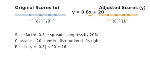
What This Problem Teaches

• Linear transformation properties: Understanding how y = ax + b affects measures of spread versus location
• Standard deviation scaling: Recognizing that standard deviation transforms by the absolute value of the coefficient
• Invariance under translation: Seeing why adding constants doesn't change variability
• Statistical reasoning: Connecting algebraic transformations to their meaning in data analysis
• Pattern recognition: Identifying when to apply transformation rules versus computing from scratch

Solution: Method 1 — The Linear Transformation Rule

When data undergoes a linear transformation of the form y = ax + b, there's a fundamental rule about how the standard deviation changes. Let's apply this principle directly.

Step 1 — Identify the transformation components

The given transformation is y = 0.8x + 20, where:
• The coefficient a = 0.8 (this scales the data)
• The constant b = 20 (this shifts the data)

Step 2 — Apply the standard deviation transformation rule

For any linear transformation y = ax + b, the new standard deviation is:

The absolute value ensures the standard deviation remains positive, and notice that the constant b doesn't appear—it only shifts the data without affecting spread.

Step 3 — Calculate the new standard deviation

Substituting our values:

Step 4 — Understand why this works

The coefficient 0.8 compresses each score toward the mean by 20%, so the spread also compresses by the same factor. The +20 shifts every score equally, preserving all the distances between scores.

Solution: Method 2 — The Variance Transformation Approach

We can also solve this by working with variance (the square of standard deviation), which follows its own transformation rule, then converting back.

Step 1 — Find the original variance

Since standard deviation is 20, the original variance is:

Step 2 — Apply the variance transformation rule

For y = ax + b, the new variance is:

Notice that the coefficient gets squared in the variance transformation.

Step 3 — Calculate the new variance

Substituting our values:

Step 4 — Convert back to standard deviation

Taking the square root of the variance:

This confirms our answer from Method 1 and shows the relationship between variance and standard deviation transformations.

Verification

Let's verify our answer by checking with a concrete example. Suppose three students had original scores of 60, 80, and 100.

Original scores: 60, 80, 100
Mean: (60 + 80 + 100) ÷ 3 = 80
Deviations: -20, 0, +20
Standard deviation: √[(20² + 0² + 20²) ÷ 3] = √[800 ÷ 3] ≈ 16.33

Adjusted scores: 0.8(60) + 20 = 68, 0.8(80) + 20 = 84, 0.8(100) + 20 = 100
New mean: (68 + 84 + 100) ÷ 3 = 84
New deviations: -16, 0, +16
New standard deviation: √[(16² + 0² + 16²) ÷ 3] = √[512 ÷ 3] ≈ 13.06

The ratio is 13.06 ÷ 16.33 ≈ 0.8, confirming our transformation rule. ✓

Watch Out For These

The Math Beneath the Surface

This problem reveals a fundamental principle about linear transformations in statistics:

This principle extends beyond test scores to any data transformation. Whether you're converting temperatures, adjusting measurements, or scaling survey responses, these rules always apply.

The key insight is that linear transformations affect location (mean) and scale (standard deviation) in predictable, separate ways. The coefficient controls scaling, while the constant controls shifting.

Why This Matters

Standardized testing: When test scores are curved or adjusted, understanding how the spread changes helps interpret the results.

Data normalization: In data science, linear transformations are used to rescale variables, and knowing how variance changes is crucial for analysis.

Quality control: Manufacturing processes often apply corrections to measurements, and predicting the resulting variability helps maintain quality standards.

What If?