




Test Scores: Normal Distribution & Empirical Rule
What This Problem Teaches
- Applying the empirical rule (68-95-99.7 rule) to real-world normal distributions
- Converting between z-scores and actual data values in context
- Translating percentages into concrete counts when dealing with populations
- Recognizing when standard deviation boundaries align with common intervals
- Building intuition for how data clusters around the mean in normal distributions
Visualizing the Normal Distribution
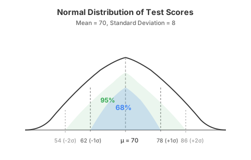
Solution: Method 1 — The Empirical Rule Approach
For normal distributions, the empirical rule provides a powerful shortcut when we're dealing with intervals that are exactly 1, 2, or 3 standard deviations from the mean.
Step 1 — Identify the given information
We have a normal distribution with:
Mean (μ) = 70Standard deviation (σ) = 8Sample size (n) = 300 studentsStep 2 — Calculate the standard deviation boundaries
Let's find what scores correspond to 1 and 2 standard deviations from the mean:
μ - 1σ = 70 - 8 = 62μ + 1σ = 70 + 8 = 78μ - 2σ = 70 - 2(8) = 54μ + 2σ = 70 + 2(8) = 86Step 3 — Apply the empirical rule
The empirical rule tells us:
- 68% of data falls within 1 standard deviation (between 62 and 78)
- 95% of data falls within 2 standard deviations (between 54 and 86)
Step 4 — Calculate the number of students
Convert percentages to actual student counts:
Students between 62-78: 68% × 300 = 0.68 × 300 = 204 studentsStudents between 54-86: 95% × 300 = 0.95 × 300 = 285 studentsSolution: Method 2 — Z-Score & Standard Normal Table
This method converts our specific values to standardized z-scores, which we can then look up in a standard normal table.
Step 1 — Convert boundaries to z-scores
Using the formula z = (x - μ)/σ:
z₁ = (62 - 70)/8 = -8/8 = -1z₂ = (78 - 70)/8 = 8/8 = +1z₃ = (54 - 70)/8 = -16/8 = -2z₄ = (86 - 70)/8 = 16/8 = +2Step 2 — Use standard normal probabilities
From the standard normal distribution:
P(-1 ≤ Z ≤ +1) = 0.6827 ≈ 68.3%P(-2 ≤ Z ≤ +2) = 0.9545 ≈ 95.4%Step 3 — Calculate student counts
Students between 62-78: 68.3% × 300 ≈ 205 studentsStudents between 54-86: 95.4% × 300 ≈ 286 studentsThis method gives slightly more precise results than the empirical rule's rounded percentages.
95% of the class (approximately 285 students) scored between 54 and 86
Verification
Let's confirm our z-score calculations and check that our intervals make sense:
| Score | Z-Score Calculation | Z-Value | Standard Deviations from Mean |
|---|---|---|---|
| 62 | (62 - 70)/8 | -1.00 | 1 below mean |
| 78 | (78 - 70)/8 | +1.00 | 1 above mean |
| 54 | (54 - 70)/8 | -2.00 | 2 below mean |
| 86 | (86 - 70)/8 | +2.00 | 2 above mean |
Sanity check: Our percentages should add up logically. Since 95% of students score between 54-86, only 5% score outside this range (below 54 or above 86). This makes sense for a normal distribution.
Common Pitfalls
Some students calculate μ ± 2σ as 70 ± 16 = 54 to 86, then incorrectly think this represents "1 standard deviation" because they're thinking of the total range. Remember: each side is 2 standard deviations from the center.
Don't memorize "68% goes with this problem" — instead, check which interval you're calculating. The 68% only applies when your boundaries are exactly μ ± 1σ. If boundaries don't align with 1σ, 2σ, or 3σ, you need z-tables or technology.
The question asks "how many students," not "what percentage." Always multiply your percentage by the total sample size: 68% × 300 = 204 students, not just "68%".
Write out your intervals clearly: 62-78 is the smaller interval (±1σ), so it gets the smaller percentage (68%). 54-86 is the larger interval (±2σ), so it gets the larger percentage (95%). The wider the net, the more students you catch.
The Pattern Behind This
This problem showcases the empirical rule, one of the most practical tools in statistics. For any normal distribution:
P(μ - 1σ ≤ X ≤ μ + 1σ) ≈ 0.68P(μ - 2σ ≤ X ≤ μ + 2σ) ≈ 0.95P(μ - 3σ ≤ X ≤ μ + 3σ) ≈ 0.997The beauty of this rule is that the actual numbers don't matter — whether you're measuring test scores, heights, weights, or manufacturing tolerances, if the data is approximately normal, these percentages remain constant.
When boundaries don't align perfectly with 1σ, 2σ, or 3σ, we need the more general approach:
z = (x - μ)/σP(a ≤ X ≤ b) = P((a-μ)/σ ≤ Z ≤ (b-μ)/σ)Where This Shows Up in Real Life
- Quality control: Manufacturing companies use these calculations to determine what percentage of products meet specifications. If bolt lengths are normally distributed with mean 5.0 cm and σ = 0.1 cm, the empirical rule tells them how many bolts fall within tolerance.
- Medical diagnostics: Blood pressure, cholesterol levels, and other biomarkers follow normal distributions. Doctors use these percentiles to determine if a patient's values are within normal ranges or require attention.
- Standardized testing: SAT, ACT, and IQ scores are designed to be normally distributed. Test makers use these principles to set score ranges and understand what percentage of test-takers achieve various performance levels.
- Financial risk management: Investment returns often approximate normal distributions. Portfolio managers use similar calculations to estimate the probability of losses exceeding certain thresholds.
What If?
For 66: z₁ = (66 - 70)/8 = -0.5
For 82: z₂ = (82 - 70)/8 = 1.5
P(Z ≤ -0.5) ≈ 0.3085P(Z ≤ 1.5) ≈ 0.9332
P(-0.5 ≤ Z ≤ 1.5) = 0.9332 - 0.3085 = 0.6247
62.47% of students score between 66 and 82 (about 187 students)
Top 16% means 84% are below this scoreP(Z ≤ z) = 0.84
From z-table: z ≈ 1.0
z = (x - μ)/σ1.0 = (x - 70)/8x = 70 + 8(1.0) = 78
A minimum score of 78 is needed for an A grade
P(Z ≤ z) = 0.84
From z-table: z ≈ 1.0
z = (x - μ)/σ1.0 = (78 - 70)/σσ = 8/1.0 = 8
The standard deviation is 8
Let D = Score_A - Score_Bμ_D = μ_A - μ_B = 70 - 75 = -5σ_D = √(σ_A² + σ_B²) = √(64 + 36) = 10
z = (0 - (-5))/10 = 0.5P(Z > 0.5) = 1 - P(Z ≤ 0.5) = 1 - 0.6915 = 0.3085
The probability is approximately 30.85%
Frequently Asked Questions
2026-11-02